Utility script for launching bare JAR files

Torsten Seemann compiled a list of minimum standards for bioinformatics command line tools, things like printing help when no commands are specified, including version info, avoid hardcoded paths, etc. These should be obvious to any seasoned software engineer, but many of these standards are not followed in bioinformatics.

#8 on the list was "Don't distribute bare JAR files." This is particularly annoying, requiring a user to invoke the software using something like: java -Xmx1000m -jar /path/on/my/system/to/software.jar . There are a few notable offenders in bioinformatics out there (I'm looking at you, Trimmomatic, snpEff, GATK...).

A very simple solution to the bare JAR file problem is distributing your java tool with a shell script wrapper that makes it easier for your users to invoke. E.g., if I have GATK installed in ~/bin/ngs/gatk/GenomeAnalysisTK.jar, I can create this shell script at ~/bin/ngs/gatk/gatk (replace GenomeAnalysisTK.jar with someOtherBioTool.jar):



Once I make that script executable and include that directory in my path, calling GATK is much simpler:


Yes, I'm fully aware that making my own JAR launcher utility scripts for existing software will make my code less reproducible, but for quick testing and development I don't think it matters. The tip has the best results when JAR files are distributed from the developer with utility scripts for invoking them.

See the post below for more standards that should be followed in bioinformatics software development.

Torsten Seeman: Minimum standards for bioinformatics command line tools

Understanding the ENSEMBL Schema

ENSEMBL is a frequently used resource for various genomics and transcriptomics tasks.  The ENSEMBL website and MART tools provide easy access to their rich database, but ENSEMBL also provides flat-file downloads of their entire database and a public MySQL portal.  You can access this using the MySQL Workbench using the following:

Host:     useastdb.ensembl.org
User:     anonymous

Once inside, you can get a sense for what the ENSEMBL schema (or data model) is like.  First, it’s important to understand the ENSEMBL ID system.  Most of the primary entities in the ENSEMBL database (genes, exons, transcripts, proteins) have a formal, stable identifier (beginning with ENSG, ENSE, ENST, and ENSP respectively) that does not change from build to build.  These entries can be found in the gene_stable_id tables.  All of these entities also have an internal identifier (an integer).  Once you have an internal ID for the entity of interest, details of the entity can be found in the genes, exons, transcripts, and translations (proteins) table. For example, the following query will retrieve a list of all transcripts and their exons for a given gene.

SELECT * FROM gene_stable_id a
inner join gene b on a.gene_id = b.gene_id
inner join transcript c on b.gene_id = c.gene_id
inner join exon_transcript d on c.transcript_id = d.transcript_id
inner join exon e on d.exon_id = e.exon_id
inner join transcript_stable_id f on c.transcript_id = f.transcript_id
inner join exon_stable_id g on e.exon_id = g.exon_id

The exon_transcript table contains a mapping of each exon to any transcripts containing it, and also contains a rank to indicate which exon it is relative to a given transcript.  To retrieve exons for a list of genes by their ENSEMBL IDs, these could be loaded into a table and joined to the gene_stable_id table in the query above.  To pull the build 37 chromosome and coordinates for an exon, use the following:

Select a.exon_id, b.name, a.seq_region_start, a.seq_region_end from exon a
inner join seq_region b on a.seq_region_id = b.seq_region_id
inner join coord_system c on b.coord_system_id = c.coord_system_id
where c.version = "GRCh37";

In this query, the seq_region table contains a field called name that identifies the contig to which the coordinates refer, in this case the chromosome number. 

There are also extensive cross-references in the ENSEMBL database.  To retrieve alternate identifiers for a set of transcripts, execute the following: 

select * from transcript_stable_id a
inner join transcript b on a.transcript_id = b.transcript_id
inner join object_xref c on b.transcript_id = c.ensembl_id
inner join xref d on c.xref_id = d.xref_id
inner join external_db e on d.external_db_id = e.external_db_id
where ensembl_object_type = "Transcript"
limit 20;

ENSEMBL organizes cross-references (xrefs) for all entity types into a single table object_xref.  This table contains an ensemble_object_type field that is a “Transcript”, “Gene”, or “Translation”, and an ensemble_id that matches either a gene_id, transcript_id, or a translation_id.  Replace “transcript” in the above query with “gene” or “translation” to retrieve gene or protein cross-references.  A list of all external cross-reference sources can be found by querying: 

Select db_name from external_db;

There is a great deal of information within the ENSEMBL database that can be accessed using SQL, which for some types of operations is easier than using the MART or web interface.  Full details of the ENSEMBL schema can be found here (http://useast.ensembl.org/info/docs/api/core/core_schema.html)

Google Developers R Programming Video Lectures

Google Developers recognized that most developers learn R in bits and pieces, which can leave significant knowledge gaps. To help fill these gaps, they created a series of introductory R programming videos. These videos provide a solid foundation for programming tools, data manipulation, and functions in the R language and software. The series of short videos is organized into four subsections: intro to R, loading data and more data formats, data processing and writing functions. Start watching the YouTube playlist here, or watch an individual lecture below:

1.1 - Initial Setup and Navigation
1.2 - Calculations and Variables
1.3 - Create and Work With Vectors
1.4 - Character and Boolean Vectors
1.5 - Vector Arithmetic
1.6 - Building and Subsetting Matrices
1.7 - Section 1 Review and Help Files
2.1 - Loading Data and Working With Data Frames
2.2 - Loading Data, Object Summaries, and Dates
2.3 - if() Statements, Logical Operators, and the which() Function
2.4 - for() Loops and Handling Missing Observations
2.5 - Lists
3.1 - Managing the Workspace and Variable Casting
3.2 - The apply() Family of Functions
3.3 - Access or Create Columns in Data Frames, or Simplify a Data Frame using aggregate()
4.1 - Basic Structure of a Function
4.2 - Returning a List and Providing Default Arguments
4.3 - Add a Warning or Stop the Function Execution
4.4 - Passing Additional Arguments Using an Ellipsis
4.5 - Make a Returned Result Invisible and Build Recursive Functions
4.6 - Custom Functions With apply()

Archival, Analysis, and Visualization of #ISMBECCB 2013 Tweets

As the 2013 ISMB/ECCB meeting is winding down, I archived and analyzed the 2000+ tweets from the meeting using a set of bash and R scripts I previously blogged about.

The archive of all the tweets tagged #ISMBECCB from July 19-24, 2013 is and will forever remain here on Github. You'll find some R code to parse through this text and run the analyses below in the same repository, explained in more detail in my previous blog post.

Number of tweets by date:

Number of tweets by hour:

Most popular hashtags, other than #ismbeccb. With separate hashtags for each session, this really shows which other SIGs and sessions were well-attended. It also shows the popularity of the unofficial ISMB BINGO card.

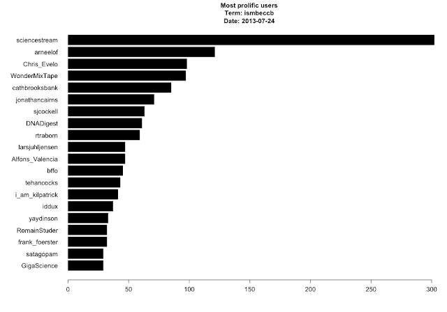
Most prolific users. I'm not sure who or what kind of account @sciencstream is - seems like spam to me.

And the obligatory word cloud:

Course Materials from useR! 2013 R/Bioconductor for Analyzing High-Throughput Genomic Data

At last week's 2013 useR! conference in Albacete, Spain, Martin Morgan and Marc Carlson led a course on using R/Bioconductor for analyzing next-gen sequencing data, covering alignment, RNA-seq, ChIP-seq, and sequence annotation using R. The course materials are online here, including R code for running the examples, the PDF vignette tutorial, and the course material itself as a package.



Course Materials from useR! 2013 R/Bioconductor for Analyzing High-Throughput Genomic Data

Customize your .Rprofile and Keep Your Workspace Clean

Like your .bashrc, .vimrc, or many other dotfiles you may have in your home directory, your .Rprofile is sourced every time you start an R session. On Mac and Linux, this file is usually located in ~/.Rprofile. On Windows it's buried somewhere in the R program files. Over the years I've grown and pruned my .Rprofile to set various options and define various "utility" functions I use frequently at the interactive prompt.

One of the dangers of defining too many functions in your .Rprofile is that your code becomes less portable, and less reproducible. For example, if I were to define adf() as a shortcut to as.data.frame(), code that I send to other folks using adf() would return errors that the adf object doesn't exist. This is a risk that I'm fully aware of in regards to setting the option stringsAsFactors=FALSE,  but it's a tradeoff I'm willing to accept for convenience. Most of the functions I define here are useful for exploring interactively. In particular, the n() function below is handy for getting a numbered list of all the columns in a data frame; lsp() and lsa() list all functions in a package, and list all objects and classes in the environment, respectively (and were taken from Karthik Ram's .Rprofile); and the o() function opens the current working directory in a new Finder window on my Mac. In addition to a few other functions that are self-explanatory, I also turn off those significance stars, set a default CRAN mirror so it doesn't ask me all the time, and source in the biocLite() function for installing Bioconductor packages (note: this makes R require web access, which might slow down your R initialization).

Finally, you'll notice that I'm creating a new hidden environment, and defining all the functions here as objects in this hidden environment. This allows me to keep my workspace clean, and remove all objects from that workspace without nuking any of these utility functions.

I used to keep my .Rprofile synced across multiple installations using Dropbox, but now I keep all my dotfiles in a single git-versioned directory, symlinked where they need to go (usually ~/). My .Rprofile is below: feel free to steal or adapt however you'd like.

ENCODE ChIP-Seq Significance Tool: Which TFs Regulate my Genes?

I collaborate with several investigators on gene expression projects using both microarray and RNA-seq. After I show a collaborator which genes are dysregulated in a particular condition or tissue, the most common question I get is "what are the transcription factors regulating these genes?"

This isn't the easiest question to answer. You could look at transcription factor binding site position weight matrices like those from TRANSFAC and come up with a list of all factors that potentially hit that site, then perform some kind of enrichment analysis on that. But this involves some programming, and is based solely on sequence motifs, not experimental data.

The ENCODE consortium spent over $100M and generated hundreds of ChIP-seq experiments for different transcription factors and histone modifications across many cell types (if you don't know much about ENCODE, go read the main ENCODE paper, and Sean Eddy's very fair commentary). Regardless of what you might consider "biologically functional", the ENCODE project generated a ton of data, and much of this data is publicly available. But that still doesn't help answer our question, because genes are often bound by multiple TFs, and TFs can bind many regions. We need to perform an enrichment (read: hypergeometric) test to assess an over-representation of experimentally bound transcription factors around our gene targets of interest ("around" also implies that some spatial boundary must be specified). To date, I haven't found a good tool to do this easily.

Raymond Auerbach and Bin Chen in Atul Butte's lab recently developed a resource to address this very common need, called the ENCODE ChIP-Seq Significance Tool.

The paper: Auerbach et al. Relating Genes to Function: Identifying Enriched Transcription Factors using the ENCODE ChIP-Seq Significance Tool. Bioinformatics (2013): 10.1093/bioinformatics/btt316.

The software: ENCODE ChIP-Seq Significance Tool (http://encodeqt.stanford.edu/).

This tool takes a list of "interesting" (significant, dysregulated, etc.) genes as input, and identifies ENCODE transcription factors from this list. Head over to http://encodeqt.stanford.edu/, select the ID type you're using (Ensembl, Symbol, etc), and paste in your list of genes. You can also specify your background set (this has big implications for the significance testing using the hypergeometric distribution). Scroll down some more to tell the tool how far up and downstream you want to look from the transcription start/end site or whole gene, select an ENCODE cell line (or ALL), and hit submit. 

You're then presented with a list of transcription factors that are most likely regulating your input genes (based on overrepresentation of ENCODE ChIP-seq binding sites). Your results can then be saved to CSV or PDF. You can also click on a number in the results table and get a list of genes that are regulated by a particular factor (the numbers do not appear as hyperlinks in my browser, but clicking the number still worked).

At the very bottom of the page, you can load example data that they used in the supplement of their paper, and run through the analysis presented therein. The lead author, Raymond Auerbach, even made a very informative screencast on how to use the tool:

Now, if I could only find a way to do something like this with mouse gene expression data.

Butte Lab: ENCODE ChIP-Seq Significance Tool  (Read the Bioinformatics paper here)