Pages

Showing posts with label ggplot2. Show all posts

Plotting the Frequency of Twitter Hashtag Usage Over Time with R and ggplot2

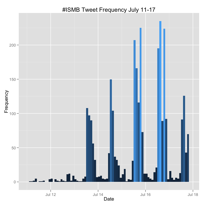
The 20th annual ISMB meeting was held over the last week in Long Beach, CA. It was an incredible meeting with lots of interesting and relevant talks, and lots of folks were tweeting the conference, usually with at least a few people in each concurrent session. I wrote the code below that uses the twitteR package to pull all the tweets about the meeting under the #ISMB hashtag. You can download that raw data here. I then use ggplot2 to plot the frequency of tweets about #ISMB over time in two hour windows for each day of the last week.

The code below also tabulates the total number of tweets by username, and plots the 40 most prolific. Interestingly several of the folks in this list weren't even at the meeting.


I'll update the plots above at the conclusion of the meeting.

Here's the code below. There's a limitation with this code - you can only retrieve a maximum of 1500 tweets per query without authenticating via OAuth before you receive a 403 error. The twitteR package had a good vignette about how to use the ROAuth package to do this, but I was never able to get it to work properly. The version on CRAN (0.9.1) has known issues, but even when rolling back to 0.9.0 or upgrading to 0.9.2 from the author's homepage, I still received the 403 signal. So my hackjob workaround was to write a loop to fetch all the tweets one day at a time and then flatten this into a single list before converting to a data frame. You still run into the limitation of only being able to retrieve the first 1500 for each day, but #ISMB never had more than 1500 any one day. If you can solve my ROAuth problem, please leave a comment or fork the code on GitHub.


Hadley Wickham: ggplot2 Webinar (Today!)


Title: A Backstage Tour of ggplot2 with Hadley Wickham
Date: Wednesday, February 8, 2012
Time: 11:00AM - 12:00PM Pacific
Presenter: Hadley Wickham, Professor of Statistics, Rice University

Register here.

I used ggplot2 extensively a few years ago, but reverted back to base graphics when ggplot2 was too slow for a project I was working on. But ggplot2 and plyr have improved much in the last few years, and I'm starting to pick it back up again. This webinar will give an overview of ggplot2, a preview of some of ggplot2's forthcoming new features, and will discuss ggplot2's internals and development over the last few years and how ggplot2 development is becoming easier.

I received an email yesterday saying that the registration list is over 1000 long, so it's a good idea to sign into the webinar early to make sure you get a spot. Hit the link below to register and you'll get a link to the webinar.

A Backstage Tour of ggplot2 with Hadley Wickham

Scatterplot matrices in R

I just discovered a handy function in R to produce a scatterplot matrix of selected variables in a dataset. The base graphics function is pairs(). Producing these plots can be helpful in exploring your data, especially using the second method below.

Try it out on the built in iris dataset. (data set gives the measurements in cm of the variables sepal length and width and petal length and width, respectively, for 50 flowers from each of 3 species of iris. The species are Iris setosa, versicolor, and virginica).

# Load the iris dataset.
data(iris)
 
# Plot #1: Basic scatterplot matrix of the four measurements
pairs(~Sepal.Length+Sepal.Width+Petal.Length+Petal.Width, data=iris)
Looking at the pairs help page I found that there's another built-in function, panel.smooth(), that can be used to plot a loess curve for each plot in a scatterplot matrix. Pass this function to the lower.panel argument of the pairs function. The panel.cor() function below can compute the absolute correlation between pairs of variables, and display these in the upper panels, with the font size proportional to the absolute value of the correlation.

# panel.smooth function is built in.
# panel.cor puts correlation in upper panels, size proportional to correlation
panel.cor <- function(x, y, digits=2, prefix="", cex.cor, ...)
{
    usr <- par("usr"); on.exit(par(usr))
    par(usr = c(0, 1, 0, 1))
    r <- abs(cor(x, y))
    txt <- format(c(r, 0.123456789), digits=digits)[1]
    txt <- paste(prefix, txt, sep="")
    if(missing(cex.cor)) cex.cor <- 0.8/strwidth(txt)
    text(0.5, 0.5, txt, cex = cex.cor * r)
}
 
# Plot #2: same as above, but add loess smoother in lower and correlation in upper
pairs(~Sepal.Length+Sepal.Width+Petal.Length+Petal.Width, data=iris,
      lower.panel=panel.smooth, upper.panel=panel.cor,
      pch=20, main="Iris Scatterplot Matrix")

Finally, you can produce a similar plot using ggplot2, with the diagonal showing the kernel density.


# Plot #3: similar plot using ggplot2
# install.packages("ggplot2") ## uncomment to install ggplot2
library(ggplot2)
plotmatrix(with(iris, data.frame(Sepal.Length, Sepal.Width, Petal.Length, Petal.Width)))


See more on the pairs function here.

...

Update:  A tip of the hat to Hadley Wickham (@hadleywickham) for pointing out two packages useful for scatterplot matrices. The gpairs package has some useful functionality for showing the relationship between both continuous and categorical variables in a dataset, and the GGally package extends ggplot2 for plot matrices.

Annotated Manhattan plots and QQ plots for GWAS using R, Revisited

Last year I showed you how to create manhattan plots, and later how to highlight regions of interest, using ggplot2 in R. The code was slow, required a lot of memory, and was difficult to maintain and modify.

I finally found time to rewrite the code using base graphics rather than ggplot2. The code is now much faster, and if you're familiar with base R's plot options and graphical parameters, most of these can now be passed to the functions to tweak the plots' appearance. The code also behaves differently depending on whether you have results for one or more than one chromosome.

Here's a quick demo.

First, either copy and paste the code from GitHub, or run the following commands in R to download and source the code from GitHub (you can't directly read from https in R, so you have to download the file first, the source it). Note the command is different on Mac vs Windows.

Download the function code on Mac:

download.file("https://raw.github.com/stephenturner/qqman/master/qqman.r", destfile="./qqman.r", method="curl")

Download the function code on Windows, leave out the method="curl" argument:

download.file("https://raw.github.com/stephenturner/qqman/master/qqman.r", destfile="./qqman.r")

Now, source the script containing the functions.

source("./qqman.r")


Next, load some GWAS results, and take a look at the relevant columns (same as above, download first then read locally from disk). This is standard output from PLINK's --assoc option.

Download example data on Mac:

download.file("https://raw.github.com/stephenturner/qqman/master/plink.assoc.txt.gz", destfile="./plink.assoc.txt.gz", method="curl")

Download example data on Windows:

download.file("https://raw.github.com/stephenturner/qqman/master/plink.assoc.txt.gz", destfile="./plink.assoc.txt.gz")

Read in the sample results, and take a look at the first few lines:

results = read.table(gzfile("./plink.assoc.txt.gz"), header=T)

head(subset(results, select=c(SNP, CHR, BP, P)))

The manhattan function assumes you have columns named SNP, CHR, BP, and P, corresponding to the SNP name (rs number), chromosome number, genomic coordinate, and p-value. Missing values (where regression failed to converge, for instance) should be recoded NA before reading into R. Do this with a quick sed command. Here's what the data looks like:

         SNP CHR        BP       P
1 rs10495434   1 235800006 0.62220
2  rs6689417   1  46100028 0.06195
3  rs3897197   1 143700035 0.10700
4  rs2282450   1 202300047 0.47280
5   rs567279   1  66400050      NA
6 rs11208515   1  64900051 0.53430


Now, create a basic manhattan plot (click the image to enlarge):

manhattan(results)


If you type args(manhattan) you can see the options you can set. Here are a few:

colors: this is a character vector specifying the colors to cycle through for coloring each point. Here's a PDF chart of R's color names.

ymax: this is the y-axis limit. If ymax="max" (default), the y-axis will always be a little bit higher than the most significant -log10(p-value). Otherwise you can set this value yourself.

cex.x.axis: this can be used to shrink the x-axis labels by setting this value less than 1. This is handy if some of the tick labels aren't showing up because the plot region is too small.

*** Update March 9 2012*** cex.x.axis is deprecated. To change the x-axis size, use the default base graphics argument cex.axis.

limitchromosomes: you can limit which chromosomes you want to display. By default this restricts the plot to chromosomes 1-23(x).

suggestiveline and genomewideline: set these to FALSE if you don't want threshold lines, or change the thresholds yourself.

annotate: by default this is undefined. If you supply a character vector of SNP names (e.g. rs numbers), any SNPs in the results data frame that also show up here will be highlighted in green by default. example below.

... : The dot-dot-dot means you can pass most other plot or graphical parameters to these functions (e.g. main, cex, pch, etc).

Make a better looking manhattan plot. Change the plot colors, point shape, and remove the threshold lines:

manhattan(results, colors=c("black","#666666","#CC6600"), pch=20, genomewideline=F, suggestiveline=F)


Now, read in a text file with SNP names that you want to highlight, then make a manhattan plot highlighting those SNPs, and give the plot a title:

Download a SNP list on Mac:

download.file("https://raw.github.com/stephenturner/qqman/master/snps.txt", destfile="./snps.txt", method="curl")

Download a SNP list on Windows:

download.file("https://raw.github.com/stephenturner/qqman/master/snps.txt", destfile="./snps.txt")

Read in the SNP list, and create an annotated plot:

snps_to_highlight = scan("./snps.txt", character())

manhattan(results, annotate=snps_to_highlight, pch=20, main="Manhattan Plot")


Finally, zoom in and plot only the results for chromosome 11, still highlighting those results. Notice that the x-axis changes from chromosome to genomic coordinate.

manhattan(subset(results, CHR==11), pch=20, annotate=snps_to_highlight, main="Chr11")


Finally, make a quantile-quantile plot of the p-values. To make a basic qq-plot of the p-values, pass the qq() function a vector of p-values:

qq(results$P)


Perhaps we should have made the qq-plot first, as it looks like we might have some unaccounted-for population stratification or other bias.

The code should run much faster and use less memory than before. All the old functions that use ggplot2 are still available, now prefixed with "gg." Please feel free to use, modify, and redistribute, but kindly link back to this post. The function source code, data, SNPs of interest, and example code used in this post are all available in the qqman GitHub repository.

Forest plots using R and ggplot2

Abhijit over at Stat Bandit posted some nice code for making forest plots using ggplot2 in R. You see these lots of times in meta-analyses, or as seen in the BioVU demonstration paper. The idea is simple - on the x-axis you have the odds ratio (or whatever stat you want to show), and each line is a different study, gene, SNP, phenotype, etc. You draw a dot for the odds ratio point estimate, and lines extending from that point showing the confidence limits for that odds ratio.

Here's the R code, slightly modified from Abhijit's version:


And here's what you get:


Thanks for sharing the code, Abhiji!

Deducer: R and ggplot2 GUI

Last Year I introduced you to R Commander, a nice graphical user interface (GUI) for R for those of you who are still hesitant to leave the clicky-box style research a la SPSS for the far more superior reproducible research using R. As most of you know I'm a huge fan of ggplot2. Many of you came to the short course Hadley Wickham gave here a few weeks ago on ggplot2 and plyr. I just came across Deducer, another GUI for R that also allows you to build plots using the ggplot2 framework using the graphical interface. See the video below and the related videos on the youtube page for a quick preview of what Deducer can do.


Deducer: Intuitive Data Analysis using R and ggplot2

Hadley Wickham's ggplot2 / Data Visualization Course Materials

Hadley Wickham, creator of ggplot2, an immensely popular framework for Tufte-friendly data visualization using R, is teaching two short courses at Vanderbilt this week. Once we opened registration to Vanderbilt students and staff we instantly filled all the available seats, so unfortunately I wasn't able to announce the course here. But the good news is that Hadley's made all the data, code, and slides from the course available online here. We weren't able to record the course, but David Smith over at Revolutions posted links to videos of Hadley teaching a similar course a few months ago.

Hadley Wickham - Visualizing Data workshop at Vanderbilt

QQ plot of p-values in R using base graphics

Update Tuesday, September 14, 2010: Fixed the ylim issue, now it sets the y axis limit based on the smallest observed p-value.

A while back Will showed you how to create QQ plots of p-values in Stata and in R using the now-deprecated sma package. A bit later on I showed you how to do the same thing in R using ggplot2. As much as we (and our readers) love ggplot2 around here, it can be quite a bit slower than using the built in base graphics. This was only recently a problem for me when I tried creating a quantile-quantile plot of over 12-million p-values. I wrote the code to do this in base graphics, which is substantially faster than using the ggplot2 code I posted a while back. The code an an example are below.


Here's what the resulting QQ-plot will look like:

Video: ggplot2 Creator Hadley Wickham's Short Course on Data Visualization Using R

Hadley Wickham, creator of ggplot2, has posted a 2 hour video on data visualization using R. You can find links to the videos and slides over at Revolutions Blog.

Check back here soon. I am working with Hadley to arrange a day-long ggplot2 short course here at Vanderbilt this summer. I'll post the date and registration info once everything is set up.

Video: Hadley Wickham gives a short course on graphics with R (via Revolutions)

Create annotated GWAS manhattan plots using ggplot2 in R

*** Update April 25, 2011: This code has gone through a major revision. Please see the updated code and tutorial here. ***

 A few months ago I showed you in this post how to use some code I wrote to produce manhattan plots in R using ggplot2. The qqman() function I described in the previous post actually calls another function, manhattan(), which has a few options you can set. I recently had to update this function to allow me to color code SNPs of interest, similar to the plots shown in figure 1 of Cristen Willer's 2008 Nature Genetics paper on lipids. I'll try to explain how to utilize that feature here.

The only extra thing you'll need here is a list of SNPs that you want to highlight. The only thing - that list of SNPs can't have the "rs" prefix on the rs numbers. They must be integers. E.g. if you want to highlight rs1234 and rs5678, you would create an array containing the integers 1234 and 5678. If you already have a list of SNPs, use the substr() command to perform a substring operation to extract only the digits from the rs numbers.

Once you load in your PLINK results and your array containing the rs numbers you want to highlight, simply call the manhattan() function with the option annotate=T, and SNPlist=x, where x is the name of the vector containing rs numbers.

Here's some example code:

# This requires ggplot2
require(ggplot2)

# First, load these functions from source:
source("http://dl.dropbox.com/u/66281/0_Permanent/qqman.r")

# Next, load your PLINK results file to a data frame:
mydata=read.table("plink.qassoc", header=TRUE)

# Assuming you already have a vector of rs numbers to highlight
head(ImportantSNPs)
[1] 3821815 1851665 1621816 1403694 1656922  166479

# Call the manhattan function, with annotate=T.
# The SNPlist argument takes the list of SNPs to highlight.
# Save the plot to an object
myplot=manhattan(mydata,annotate=T,SNPlist=ImportantSNPs)

# Finally, save the plot in the current directory using ggsave()
ggsave("manhattan.png",myplot,w=12,h=9,dpi=100)

If all goes well, you should have a manhattan plot with SNPs of interest highlighted. It might look something like this:

A few tips: You can use the UCSC genome browser to look up coordinates for genes, then select rs numbers based on that range, if you want to highlight certain genes. The default color is green but you can change this on line 118 of the code at the URL above.

*** Update April 25, 2011: This code has gone through a major revision. Please see the updated code and tutorial here. ***

Arrange multiple ggplot2 plots in the same image window

In a previous tutorial I showed you how to create plots faceted by the level of a third variable using ggplot2. A commenter asked about using faceted plots and viewports and reminded me of this function I found in the ggplot2 Google group. The arrange function below is similar to using par(mfrow=c(r,c)) in base graphics to put more than one plot in the same image window.


The basic idea is that you assign ggplot2 plots to an object, and then use the arrange function to display two or more. Here's an example. First copy and paste the code above (or put in your Rprofile). Next install and/or load ggplot2 as described in a previous ggplot2 tutorial.

# Load the diamonds dataset
data(diamonds)

# Create a histogram, assign to "plot1"
plot1 <- qplot(price,data=diamonds,binwidth=1000)

# Create a scatterplot
plot2 <- qplot(carat,price,data=diamonds)

# Arrange and display the plots into a 2x1 grid
arrange_ggplot2(plot1,plot2,ncol=1)
And here's what you should get:


...

Fluctuation plot using ggplot2 in R

Found this nice way to visually summarize contingency tables using ggplot2 in R on Hadley Wickham's ggplot2 cheat sheet. Using the same data in my previous post on making scatterplots in small multiples, I'll demonstrate how to use ggfluctuation() to make a fluctuation plot. For a two-dimensional table, this simply puts different dimensions on the x and y axes, and the area of the rectangles is proportional to the density of observations in that cell of the table. Install ggplot2 as in the previous post, and run this code.
# Load ggplot2. Use install.packages("ggplot2") if you do not already have ggplot2 installed.
library(ggplot2)

# Load the diamonds dataset.
data(diamonds)

# Look at a few rows of the relevant columns
diamonds[1:20,2:3]

# Display the contingency table
table(diamonds$cut,diamonds$color)

# Make the fluctuation plot
ggfluctuation(table(diamonds$cut,diamonds$color))


The table looks like this:

             D    E    F    G    H    I    J
Fair       163  224  312  314  303  175  119
Good       662  933  909  871  702  522  307
Very Good 1513 2400 2164 2299 1824 1204  678
Premium   1603 2337 2331 2924 2360 1428  808
Ideal     2834 3903 3826 4884 3115 2093  896

And the plot:


As a side note, I'm experimenting with a new way to post R code. If you hover your mouse over the code above you can click this button to copy all the text to your clipboard.

GWAS Manhattan plots and QQ plots using ggplot2 in R

*** Update April 25, 2011: This code has gone through a major revision. Please see the updated code and tutorial here. ***

Will posted earlier this week about how to produce manhattan plots of GWAS results using Stata, so I thought I'd share how I do this in R using ggplot2.

First, if you've never used ggplot2, you'll need to add it to your R installation by typing:

install.packages("ggplot2")

Once you've done that, copy and paste this command to download the functions I wrote necessary to produce these plots.  If you'd like to see the source code yourself, copy the URL into your web browser.

source("http://dl.dropbox.com/u/66281/0_Permanent/qqman.r")

Next, read in the PLINK results file to a data frame. Substitute plink.qassoc with your own results filename.

mydata=read.table("plink.qassoc", header=TRUE)

Finally, run this function which will produce and save in the current directory both a QQ-plot and a manhattan plot of your results:

qqman(mydata)

QQ-Plot (these are simulated GWAS results):


Manhattan plot (click to enlarge):

A few notes:  First, if you're doing this on a linux machine from your Windows computer, you'll need to be running the previously mentioned XMing server on your Windows computer for the plot to save correctly.  Second, the qqman() function calls the manhattan() function, which is extremely slow and memory-intensive. It may take about 3 minutes to run for each dataset. The memory issue isn't a problem on 64-bit machines, but you may run out of memory on 32-bit machines if you're doing this with GWAS data. I'm going to try to improve this in the future. Finally, using that source command you also downloaded a function I wrote called qqmanall(), which does just what it sounds like - if you run it on a linux machine with no arguments it reads in ALL of the plink GWAS results stored in the current directory, and creates QQ and manhattan plots for all of them with a common upper limit for the y-axis corresponding to the most significant result. Enjoy.

...

Update Thursday, January 21, 2010: I neglected to mention yesterday the format of the plink.assoc or plink.qassoc files, in case you want to produce the same plots using results from another software other than plink. When you load your .assoc files in a data frame, the relevant columns are named "CHR", "BP", and "P". You can use this plotting function as long as you have these three columns in your data frame, regardless of whether you use PLINK or not.

The latest version of the code is reproduced below:

*** Update April 25, 2011: This code has gone through a major revision. Please see the updated code and tutorial here. ***


...

*** Update April 25, 2011: This code has gone through a major revision. Please see the updated code and tutorial here. ***

ggplot2 Tutorial: Scatterplots in a Series of Small Multiples

It took several months after learning about ggplot2 before I gave it a try myself.  I was apprehensive about learning a new graphics system with a new set of commands.  Thing is, if you've ever used plot() in R, you already know how to use much of the functionality in ggplot2!  In this tutorial I want to show you just how easy it is to start producing high-quality graphics using ggplot2.  I'll also introduce the concept of a series of small multiples, and show you how ggplot2 makes it dead simple to produce these kinds of graphics yourself.

Getting started:

First of all, if you've never used ggplot2 before, you'll need to download and install it.  Fire up R, and type this command, exactly as is, with the quotes:

install.packages("ggplot2")

Pick a mirror that's close to you, and install.  Once you do this, or if you've already installed ggplot2 in the past, load the ggplot2 library (no quotes this time).  You'll have to do this every time you start a new R session.

library(ggplot2)

Now we need some data.  Rather than making up our own data, let's use the "diamonds" dataset that comes packaged with ggplot2. Type this command:

data(diamonds)

This dataset contains ~50,000 entries.  Each row is an individual diamond, and some of the variables of interest include the weight of the diamond in carats, color, clarity, and its price. We can get a very good picture of the relationship between these variables using some fairly simple plotting commands.  First let's take a look at the first few rows of the dataset using the head() function.

head(diamonds)

Here's what the first few rows of the relevant columns look like:

   carat price color clarity
1   0.23   326     E     SI2
2   0.21   326     E     SI1
3   0.23   327     E     VS1
4   0.29   334     I     VS2
5   0.31   335     J     SI2
6   0.24   336     J    VVS2
7   0.24   336     I    VVS1
8   0.26   337     H     SI1
9   0.22   337     E     VS2
10  0.23   338     H     VS1


The variables carat and price are both continuous variables, while color and clarity are discrete, or in R lingo, factor variables.  Wikipedia has nice charts describing what these codes mean for a diamond's color and clarity.

First, let's take a look at the distribution of price using a histogram.

Using base graphics:

with(diamonds, hist(price))

 And using the qplot function ggplot2:

qplot(price, data=diamonds)


You may have gotten a warning that you didn't specify the bin width.  Hadley Wickham, ggplot2's creator, seems like a nice guy.  He encourages you to specify how wide you want the bins, but even if you don't, ggplot2 will still make your plot using sensible defaults.  Let's specify the binwidth ourselves this time:

qplot(price, data=diamonds, binwidth=1000)


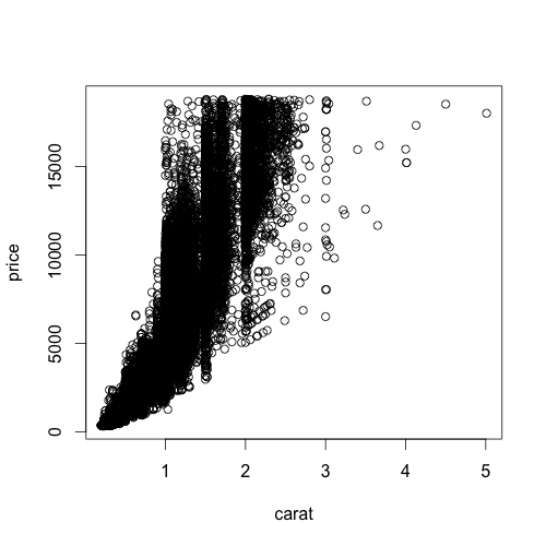
That plot looks a lot like the defaults using base graphics.  Now let's take a look at the relationship between the price of a diamond and its weight in carats.

Using base graphics:

with(diamonds, plot(carat,price))


And using ggplot2:

qplot(carat, price, data=diamonds)


Notice something about the ggplot2 syntax here. Using base R graphics there are different commands for scatterplots and histograms. But in ggplot2, if you specify a single continuous variable to the qplot command, you'll get a histogram. If you specify two continuous variables to the same qplot command, you get a scatterplot. The bars in a histogram and the points on a scatterplot are called "geoms" in ggplot2 lingo.  You can specify exactly which geom you want to use, but since Hadley's such a nice guy, ggplot2 will often guess which type of "geom" you want to use based on the data type you give it.  Let's say you wanted to look at the distribution of price using the kernel density estimation, rather than a histogram.  The command is very similar to the command you used to get a histogram, you just specify "density" as the geom, instead of leaving this option out:

qplot(price, data=diamonds, geom="density")


As you can see, using different types of "geoms" with different data types allows you to break many graphical conventions. This is usually a bad thing, but this also allows you to be creative and design your own way to display data.  Anyhow, let's get back to scatterplots.

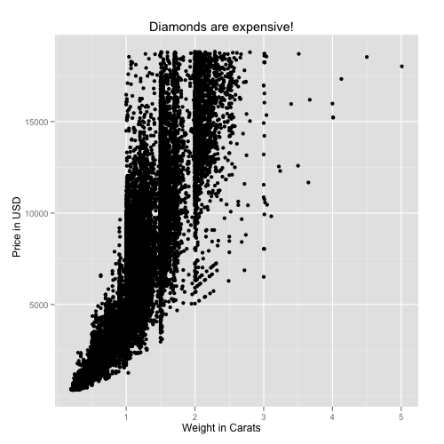
Let's say you want to add labels and a main title to your plot using xlab, ylab, and main.  If you know how to do this using base graphics, then you already know how to do this using ggplot2.

Using base graphics:
with(diamonds, plot(carat,price, xlab="Weight in Carats", ylab="Price in USD", main="Diamonds are expensive!"))


And using ggplot2:
qplot(carat, price, data=diamonds, xlab="Weight in Carats", ylab="Price in USD", main="Diamonds are expensive!")


All we've done so far is to examine the relationship between carat and price.  As one would expect, the price increases sharply as the size of the diamond increases.  But what about the other variables here, color and clarity? Specifically, does color or clarity modify the effect of carat on price? In other words, is there an interaction between carat and either of these variables?

To visualize this graphically, we could plot price vs carat for each level of one of the other two vactors, color or clarity. In ggplot2 terminology, we could facet the plot by one of these factor variables. Let's look at color first. The facets option does just this.  The syntax "color~." is saying that we want plots of price vs carat by color, where color is on the rows.  If you wanted separate facets beside each other in columns, the syntax would look like ".~color".

qplot(carat, price, data=diamonds, facets=color~.)


This plot reveals something important about the relationship between these three variables.  As the letters go from D to J, the diamond becomes more and more yellow.  This plot shows us that as the diamond's color becomes more white, an increase in carat causes a faster increase in price.  In other words, the color of the diamond modifies the effect of carat.

We can formally test in linear regression using the lm (linear model) command.  Note that I'm treating color now as a continuous (numeric) variable.  The output shows us that the interaction is significant at p<2e-16.

fit1=lm(price~carat*as.numeric(color), data=diamonds)
summary(fit1)

Call:
lm(formula = price ~ carat * as.numeric(color), data = diamonds)

Residuals:
      Min        1Q    Median        3Q       Max
-15445.88   -813.27    -20.89    634.69  11740.29

Coefficients:
                         Estimate Std. Error t value Pr(>|t|)   
(Intercept)             -2532.529     29.871 -84.782   <2e-16 ***
carat                    9276.490     35.789 259.202   <2e-16 ***
as.numeric(color)          -3.227      7.445  -0.433    0.665   
carat:as.numeric(color)  -298.153      7.777 -38.340   <2e-16 ***
---
Signif. codes:  0 ‘***’ 0.001 ‘**’ 0.01 ‘*’ 0.05 ‘.’ 0.1 ‘ ’ 1

Residual standard error: 1476 on 53936 degrees of freedom
Multiple R-squared: 0.8631,     Adjusted R-squared: 0.8631
F-statistic: 1.134e+05 on 3 and 53936 DF,  p-value: < 2.2e-16

You can also do the same thing for clarity (omitting the statistical analysis):

qplot(carat, price, data=diamonds, facets=clarity~.)


As you go down the panels the diamond gets more and more clear.  The numbers beside "S" (small) and "VS" (very small) describe the size of the "inclusions", or internal imperfections, in the stones. "IF" means internally flawless, a rare find.  As you'd expect, as the diamond becomes more and more flawless, the price per carat dramatically increases.

Finally, as you'd imagine, you can facet by both color and clarity, one on the columns and one on the rows.  You'll have to click on the image below to see it full-screen.

qplot(carat, price, data=diamonds, facets=clarity~color)


The bottom left panel shows price vs carat for very white, internally flawless diamonds.  Notice how few observations are in this cell compared to others.  These are extremely rare and expensive stones.  Compare the relationship here with the relationship in the upper right facet, where you have the yellowest, and dirtiest diamonds. You can statistically test this one as well, and you'll find that there's a highly significant (p<1e-16) three-way interaction between carat, color, and clarity, that influences the price of the diamond.

This last plot above brings me to the topic in the title, "small multiples." This term, popularized by Edward Tufte, refers to visually displaying relationships in data using the same type of figure over and over again.  The idea here is that you teach the reader once how to interpret each individual component.  Once the reader is oriented to a single component, you can show small multiples of the same figure over and over again to display how relationships change based on certain factors, without requiring the reader to figure out how to decode a new graphic every time. The fact that the figure above distills 215,760 data points across 4 dimensions into a graphic that you can interpret within seconds proves that using small multiples can be a highly effective way to display large, high-dimensional data. Do an image search for small multiples to see many more examples.  Tufte is cited in chapter 1 of the ggplot2 book, and it's very adept at displaying complex relationships in big data in an intuitive and effective manner.

I only used this diamonds dataset because it's free and readily available once you install ggplot2. There are so many ways you can use this technique for data visualization in genetics, where interactions between variables and their influence on traits are difficult to ignore.  I hope I've convinced you that using ggplot2 is no harder than base graphics, and makes high-dimensional plotting very easy. If you've found this tutorial useful, let me know in the comments, and I'll try to post a few more like this later on.

New Features in ggplot2 0.8.5

Learning R blog details some of the new features in the latest update to ggplot2. The latest version includes functions to make it easier to change axis and legend labels, as well as a function to easily set the limits of the plot display outside the range of the data.

Be sure to check back next week - I'm putting together a short introductory ggplot2 tutorial.

QQ plots of p-values in R using ggplot2

Way back will wrote on this topic.  See his previous post for Stata code for doing this.  Unfortunately the R package that was used to create QQ-plots here has been removed from CRAN, so I wrote my own using ggplot2 and some code I received from Daniel Shriner at NHGRI.

Of course you can use R's built-in qqplot() function, but I could never figure out a way to add the diagonal using base graphics.  To get the function I wrote to make qqplots, copy and paste this into your R session:

qq = function(pvector, title="Quantile-quantile plot of p-values", spartan=F) {
    # Thanks to Daniel Shriner at NHGRI for providing this code for creating expected and observed values
    o = -log10(sort(pvector,decreasing=F))
    e = -log10( 1:length(o)/length(o) )
    # you could use base graphics
    #plot(e,o,pch=19,cex=0.25, xlab=expression(Expected~~-log[10](italic(p))), ylab=expression(Observed~~-log[10](italic(p))),xlim=c(0,max(e)),ylim=c(0,max(e)))
    #lines(e,e,col="red")
    #You'll need ggplot2 installed to do the rest
    plot=qplot(e,o, xlim=c(0,max(e)), ylim=c(0,max(o))) + stat_abline(intercept=0,slope=1, col="red")
    plot=plot+opts(title=title)
    plot=plot+scale_x_continuous(name=expression(Expected~~-log[10](italic(p))))
    plot=plot+scale_y_continuous(name=expression(Observed~~-log[10](italic(p))))
    if (spartan) plot=plot+opts(panel.background=theme_rect(col="grey50"), panel.grid.minor=theme_blank())
    plot
}


Also, make sure you have ggplot2 installed:

install.packages("ggplot2")

If you already have it installed, load it:

library(ggplot2)

The function takes a vector of p-values, optionally a title, and a third option to make the plot black and white.  You can check the default arguments to the function by typing args(qq).

qq(data$Pvals, title="My Quantile-Quantile Plot")


You can also make the plot more "Spartan" by removing the title (setting it to NULL) and by making the color scheme black on white:

qq(data$Pvals, title=NULL, spartan=TRUE)


Stay tuned - I'm also putting together a way to import your PLINK output files and make better Manhattan plots using R and ggplot2 than you ever could with Haploview.

Update Tuesday, November 10, 2009: A big tip of the hat to the anonymous commenter who pointed out that this can easily be done in the base graphics package, as well as adding confidence intervals.  As always, we welcome your comments if you know of a better or easier way to do anything mentioned here!

Visualizing sample relatedness in a GWAS using PLINK and R

Strict quality control procedures are extremely important for any genome-wide association study.  One of the first steps you should take when running QC on your GWAS is to look for related samples in your dataset.  This does two things for you.  First, you can get an idea of how many related samples you have in your dataset, and second, if you have access to self-report relationship information, you can identify potential sample mix-ups based on discrepancies between genetic information and self-report.

PLINK allows you to estimate genomewide IBD-sharing coefficients between seemingly unrelated individuals from whole-genome data.  You can read lots more about the particular method they use to infer IBD given IBS and allele frequencies in the PLINK paper.  It's relatively straightforward to compute these estimates.  If you already have your data in pedfile format, use the following command (assuming mydata.ped and mydata.map are in the current directory where you run PLINK).

plink --file mydata --genome --min 0.05

This will usually take a few days if you use genome-wide data.  You could speed this up by first thinning your dataset to around 100,000 markers using the --thin option to create a smaller dataset.

After you've run this you'll have a file in that directory called plink.genome.  You can read about the output here, but we're really interested in Z1 and Z0, the proportion of markers identical by descent 1 and 0 respectively, for every pair of individuals in the dataset.  You can plot Z1 by Z0 and color code them by the relationship type as coded in the pedfile using this R code.

Here's what the columns of interest will look like:

  RT     Z1     Z0
1 UN 0.1697 0.8294
2 OT 0.5034 0.4879
3 OT 0.4403 0.5439
4 OT 0.5200 0.4674
5 UN 0.1646 0.8311
6 OT 0.5519 0.4481


First, fire up R, go to the directory where your plink results are located and load in the data:

d = read.table("plink.genome", header=T)

Next, set up the plot area. The par option makes the points solid instead of an open circle, and the plot command sets up your plot and axes without adding any points.

par(pch=16)
with(d,plot(Z0,Z1, xlim=c(0,1), ylim=c(0,1), type="n"))

Your plot should be empty, like this:


Now use this command to plot points where the relationship type is FS, or full sibling.  Make the points green (col=3).

with(subset(d,RT=="FS") , points(Z0,Z1,col=3))


Do the same thing with half sibs, "other related" (have the same family ID), parent offspring pairs, and unrelated, making each of them a different color.

with(subset(d,RT=="HS") , points(Z0,Z1,col="darkorange"))
with(subset(d,RT=="OT") , points(Z0,Z1,col=4))
with(subset(d,RT=="PO") , points(Z0,Z1,col=2))
with(subset(d,RT=="UN") , points(Z0,Z1,col=1))


You might want to rerun the commands for "other related" and especially half sibs, because they were covered up when you plotted unrelateds.

with(subset(d,RT=="OT") , points(Z0,Z1,col=4))
with(subset(d,RT=="HS") , points(Z0,Z1,col="darkorange"))


Finally, add a legend

legend(1,1, xjust=1, yjust=1, legend=levels(d$RT), pch=16, col=c(3,"darkorange",4,2,1))


For a recap, your code should look like this:


d = read.table("plink.genome", header=T)

par(pch=16)
with(d,plot(Z0,Z1, xlim=c(0,1), ylim=c(0,1), type="n"))

with(subset(d,RT=="FS") , points(Z0,Z1,col=3))
with(subset(d,RT=="HS") , points(Z0,Z1,col="darkorange"))
with(subset(d,RT=="OT") , points(Z0,Z1,col=4))
with(subset(d,RT=="PO") , points(Z0,Z1,col=2))
with(subset(d,RT=="UN") , points(Z0,Z1,col=1))
with(subset(d,RT=="OT") , points(Z0,Z1,col=4))
with(subset(d,RT=="HS") , points(Z0,Z1,col="darkorange"))

legend(1,1, xjust=1, yjust=1, legend=levels(d$RT), pch=16, col=c(3,"darkorange",4,2,1))


What you can see from the above plot is that self-reported parent-offspring pairs share 100% of their alleles IBD=1.  There is a single sib pair at the bottom left where Pr(IBD=1)=0 and Pr(IBD=0)=0.  This means that this sib pair shares 2 alleles identical by descent at every locus across the genome.  This is either a duplicated sample or a set of identical twins.  The full sibs cluster right around the middle of the plot, and you have lots of unrelated or "other related" pairs stretching from completely unrelated (bottom right quadrant) to relatively closely related (2nd or 3rd degree relatives, right around the middle of the plot).  If you see self-reported sibs showing up where the unrelated individuals cluster on this plot, or vice versa, this should clue you in on potential sample identity problems.

...

Just for fun, let's make the same plot using ggplot2.  Make sure you have the data loaded as above, then install ggplot2 if you haven't already

install.packages("ggplot2")

You only have to install the package once.  Next load the package:

library(ggplot2)

Use this incredibly simple command to make the plot:

qplot(Z0,Z1,data=d,colour=RT)


I'm not a huge fan of these colors, so lets make them the same as above:

qplot(Z0,Z1,data=d,colour=RT) + scale_colour_manual(value=c(3,"darkorange",4,2,1))


That's a little better.  Obviously the code to do this is MUCH simpler in ggplot2.  The only problem I have with this is that it automatically plots the points in the order of the levels of RT, ie. FS, then HS, then OT, PO, then UN, so you end up covering up all your half-sibs with "other related" and unrelated pairs.  Post a comment if you know how to go back and replot the HS points over the UN points.  For more on ggplot2, see my previous post comparing histograms made using Stata, R base, R lattice and R ggplot2.

Comparison of plots using Stata, R base, R lattice, and R ggplot2, Part I: Histograms

One of the nicer things about many statistics packages is the extremely granular control you get over your graphical output.  But I lack the patience to set dozens of command line flags in R, and I'd rather not power the computer by pumping the mouse trying to set all the clicky-box options in Stata's graphics editor.  I want something that just looks nice, using the out-of-the-box defaults.  Here's a little comparison of 4 different graphing systems (three using R, and one using Stata) and their default output for plotting a histogram of a continuous variable split over three levels of a categorical variable.

First I'll start with the three graphing systems in R: base, lattice, and ggplot2.  If you don't have the last two packages installed, go ahead and download them:

install.packages("ggplot2")
install.packages("lattice")

Now load these two packages, and download this fake dataset I made up containing 100 samples each from three different genotypes ("geno") and a continuous outcome ("trait")

mydat=read.csv("http://people.vanderbilt.edu/~stephen.turner/ggd/2009-09-21-histodemo.csv",header=T)
library(ggplot2)
library(lattice)

Now let's get started...

R: base graphics

par(mfrow=c(3,1))
with(subset(mydat,geno=="aa"),hist(trait))
with(subset(mydat,geno=="Aa"),hist(trait))
with(subset(mydat,geno=="AA"),hist(trait))


R: lattice

histogram(~trait | factor(geno), data=mydat, layout=c(1,3))


R: ggplot2

qplot(trait,data=mydat,facets=geno~.)

# Update Tuesday, September 22, 2009
# A commenter mentioned that this code did not work.
# If the above code does not work, try explicitly
# stating that you want a histogram:
qplot(trait,geom="histogram",data=mydat,facets=geno~.)


Stata

insheet using "http://people.vanderbilt.edu/~stephen.turner/ggd/2009-09-21-histodemo.csv", comma clear
histogram trait, by(geno, col(1))


Commentary

In my opinion ggplot2 is the clear winner.  Again I'll concede that all of the above graphing systems give you an incredible amount of control of every aspect of the graph, but I'm only looking for what gives me the best out-of-the-box default plot using the shortest command possible. R's base graphics give you a rather spartan plot, with very wide bins.  It also requires 4 lines of code.  (If you can shorten this, please comment).  By default, the base graphics system gives you counts (frequency) on the vertical axis.  The lattice package in R does a little better perhaps, but the default color scheme is visually less than stellar.  Also, I'm not sure why the axis labels switch sides every other plot, and the ticks on top of the plot are probably unnecessary.  I still think the bins are too wide.  You lose some information especially on the bottom plot towards the right tail.  The vertical axis is proportion of total.  Stata's default plot looks very similar to lattice, but again uses a very unattractive color scheme.  It uses density for the vertical axis, which may not mean much to non-statisticians.  The default plot made by ggplot2 is just hands-down good-looking.  There are no unnecessary lines delimiting the bins, and the binwidth is appropriate.  The vertical axis represents counts.  The black bars on the light-gray background have a good data-ink ratio.  And it required the 2nd shortest command, only 3 characters longer than the Stata equivalent.

I'm ordering the ggplot2 book (Amazon, ~$50), so as I figure out how to do more with ggplot2 I'll post more comparisons like this.  If you use SPSS, SAS, MATLAB, or something else, post the code in a comment here and send me a picture or link to the plot and I'll post it here.