


Google Developers recognized that most developers learn R in bits and pieces, which can leave significant knowledge gaps. To help fill these gaps, they created a series of introductory R programming videos. These videos provide a solid foundation for programming tools, data manipulation, and functions in the R language and software. The series of short videos is organized into four subsections: intro to R, loading data and more data formats, data processing and writing functions. Start watching the YouTube playlist here, or watch an individual lecture below:
1.1 - Initial Setup and Navigation
1.2 - Calculations and Variables
1.3 - Create and Work With Vectors
1.4 - Character and Boolean Vectors
1.5 - Vector Arithmetic
1.6 - Building and Subsetting Matrices
1.7 - Section 1 Review and Help Files
2.1 - Loading Data and Working With Data Frames
2.2 - Loading Data, Object Summaries, and Dates
2.3 - if() Statements, Logical Operators, and the which() Function
2.4 - for() Loops and Handling Missing Observations
2.5 - Lists
3.1 - Managing the Workspace and Variable Casting
3.2 - The apply() Family of Functions
3.3 - Access or Create Columns in Data Frames, or Simplify a Data Frame using aggregate()
4.1 - Basic Structure of a Function
4.2 - Returning a List and Providing Default Arguments
4.3 - Add a Warning or Stop the Function Execution
4.4 - Passing Additional Arguments Using an Ellipsis
4.5 - Make a Returned Result Invisible and Build Recursive Functions
4.6 - Custom Functions With apply()
Showing posts with label R. Show all posts
Showing posts with label R. Show all posts
Archival, Analysis, and Visualization of #ISMBECCB 2013 Tweets
As the 2013 ISMB/ECCB meeting is winding down, I archived and analyzed the 2000+ tweets from the meeting using a set of bash and R scripts I previously blogged about.
The archive of all the tweets tagged #ISMBECCB from July 19-24, 2013 is and will forever remain here on Github. You'll find some R code to parse through this text and run the analyses below in the same repository, explained in more detail in my previous blog post.
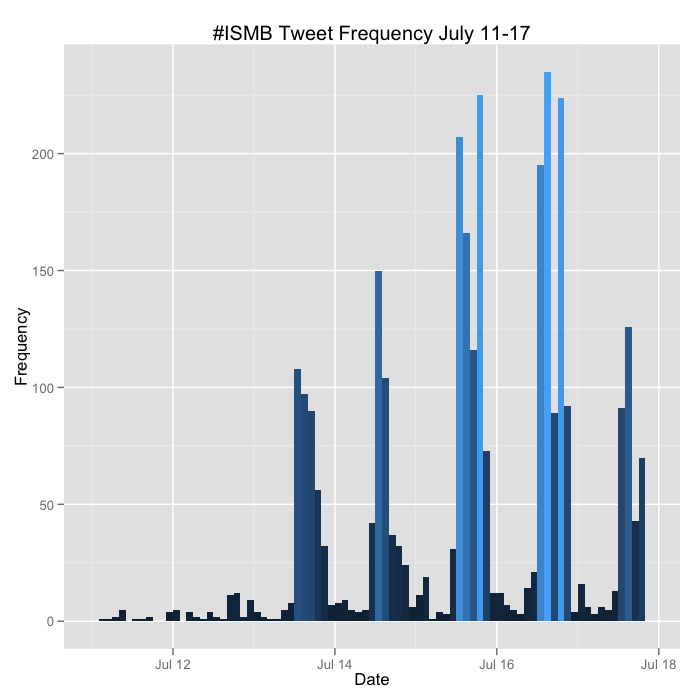
Number of tweets by date:

Number of tweets by hour:

Most popular hashtags, other than #ismbeccb. With separate hashtags for each session, this really shows which other SIGs and sessions were well-attended. It also shows the popularity of the unofficial ISMB BINGO card.

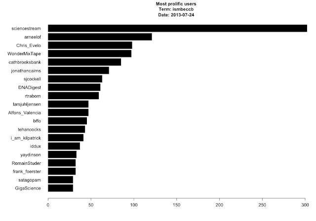
Most prolific users. I'm not sure who or what kind of account @sciencstream is - seems like spam to me.
And the obligatory word cloud:

The archive of all the tweets tagged #ISMBECCB from July 19-24, 2013 is and will forever remain here on Github. You'll find some R code to parse through this text and run the analyses below in the same repository, explained in more detail in my previous blog post.
Number of tweets by date:

Number of tweets by hour:

Most popular hashtags, other than #ismbeccb. With separate hashtags for each session, this really shows which other SIGs and sessions were well-attended. It also shows the popularity of the unofficial ISMB BINGO card.

Most prolific users. I'm not sure who or what kind of account @sciencstream is - seems like spam to me.

And the obligatory word cloud:

Course Materials from useR! 2013 R/Bioconductor for Analyzing High-Throughput Genomic Data
At last week's 2013 useR! conference in Albacete, Spain, Martin Morgan and Marc Carlson led a course on using R/Bioconductor for analyzing next-gen sequencing data, covering alignment, RNA-seq, ChIP-seq, and sequence annotation using R. The course materials are online here, including R code for running the examples, the PDF vignette tutorial, and the course material itself as a package.
Course Materials from useR! 2013 R/Bioconductor for Analyzing High-Throughput Genomic Data
Course Materials from useR! 2013 R/Bioconductor for Analyzing High-Throughput Genomic Data
Customize your .Rprofile and Keep Your Workspace Clean
Like your .bashrc, .vimrc, or many other dotfiles you may have in your home directory, your .Rprofile is sourced every time you start an R session. On Mac and Linux, this file is usually located in ~/.Rprofile. On Windows it's buried somewhere in the R program files. Over the years I've grown and pruned my .Rprofile to set various options and define various "utility" functions I use frequently at the interactive prompt.
One of the dangers of defining too many functions in your .Rprofile is that your code becomes less portable, and less reproducible. For example, if I were to define adf() as a shortcut to as.data.frame(), code that I send to other folks using adf() would return errors that the adf object doesn't exist. This is a risk that I'm fully aware of in regards to setting the option stringsAsFactors=FALSE, but it's a tradeoff I'm willing to accept for convenience. Most of the functions I define here are useful for exploring interactively. In particular, the n() function below is handy for getting a numbered list of all the columns in a data frame; lsp() and lsa() list all functions in a package, and list all objects and classes in the environment, respectively (and were taken from Karthik Ram's .Rprofile); and the o() function opens the current working directory in a new Finder window on my Mac. In addition to a few other functions that are self-explanatory, I also turn off those significance stars, set a default CRAN mirror so it doesn't ask me all the time, and source in the biocLite() function for installing Bioconductor packages (note: this makes R require web access, which might slow down your R initialization).
Finally, you'll notice that I'm creating a new hidden environment, and defining all the functions here as objects in this hidden environment. This allows me to keep my workspace clean, and remove all objects from that workspace without nuking any of these utility functions.
I used to keep my .Rprofile synced across multiple installations using Dropbox, but now I keep all my dotfiles in a single git-versioned directory, symlinked where they need to go (usually ~/). My .Rprofile is below: feel free to steal or adapt however you'd like.
Automated Archival and Visual Analysis of Tweets Mentioning #bog13, Bioinformatics, #rstats, and Others
Automatically Archiving Twitter Results
Ever since Twitter gamed its own API and killed off great services like IFTTT triggers, I've been looking for a way to automatically archive tweets containing certain search terms of interest to me. Twitter's built-in search is limited, and I wanted to archive interesting tweets for future reference and to start playing around with some basic text / trend analysis.
Enter t - the twitter command-line interface. t is a command-line power tool for doing all sorts of powerful Twitter queries using the command line. See t's documentation for examples.
I wrote this script that uses the t utility to search Twitter separately for a set of specified keywords, and append those results to a file. The comments at the end of the script also show you how to commit changes to a git repository, push to GitHub, and automate the entire process to run twice a day with a cron job. Here's the code as of May 14, 2013:
That script, and results for searching for "bioinformatics", "metagenomics", "#rstats", "rna-seq", and "#bog13" (the Biology of Genomes 2013 meeting) are all in the GitHub repository below. (Please note that these results update dynamically, and searching Twitter at any point could possibly result in returning some unsavory Tweets.)
https://github.com/stephenturner/twitterchive
Analyzing Tweets using R
You'll also find an analysis subdirectory, containing some R code to produce barplots showing the number of tweets per day over the last month, frequency of tweets by hour of the day, the most used hashtags within a search, the most prolific tweeters, and a ubiquitous word cloud. Much of this code is inspired by Neil Saunders's analysis of Tweets from ISMB 2012. Here's the code as of May 14, 2013:
Also in that analysis directory you'll see periodically updated plots for the results of the queries above.
Analyzing Tweets mentioning "bioinformatics"
Using the bioinformatics query, here are the number of tweets per day over the last month:

Here is the frequency of "bioinformatics" tweets by hour:
 Here are the most used hashtags (other than #bioinformatics):
 Here are the most prolific bioinformatics Tweeps:
 Here's a wordcloud for all the bioinformatics Tweets since March:
 Analyzing Tweets mentioning "#bog13"
The 2013 CSHL Biology of Genomes Meeting took place May 7-11, 2013. I searched and archived Tweets mentioning #bog13 from May 1 through May 14 using this script. You'll notice in the code above that I'm no longer archiving this hashtag. I probably need a better way to temporarily add keywords to the search, but I haven't gotten there yet.
Here are the number of Tweets per day during that period. Tweets clearly peaked a couple days into the meeting, with follow-up commentary trailing off quickly after the meeting ended.

Here is the frequency frequency of Tweets by hour, clearly bimodal:
 Top hashtags (other than #bog13). Interestingly #bog14 was the most highly used hashtag, so I'm guessing lots of folks are looking forward to next years' meeting. Also, #ashg12 got lots of mentions, presumably because someone presented updated work from last years' ASHG meeting.
 Here were the most prolific Tweeps - many of the usual suspects here, as well as a few new ones (new to me at least):
 And finally, the requisite wordcloud:

More analysis
If you look in the analysis directory of the repo you'll find plots like these for other keywords (#rstats, metagenomics, rna-seq, and others to come). I would also like to do some sentiment analysis as Neil did in the ISMB post referenced above, but the sentiment package has since been removed from CRAN. I hear there are other packages for polarity analysis, but I haven't yet figured out how to use them. I've given you the code to do the mundane stuff (parsing the fixed-width files from t, for starters). I'd love to see someone take a stab at some further text mining / polarity / sentiment analysis!
twitterchive - archive and analyze results from a Twitter search
Ever since Twitter gamed its own API and killed off great services like IFTTT triggers, I've been looking for a way to automatically archive tweets containing certain search terms of interest to me. Twitter's built-in search is limited, and I wanted to archive interesting tweets for future reference and to start playing around with some basic text / trend analysis.
Enter t - the twitter command-line interface. t is a command-line power tool for doing all sorts of powerful Twitter queries using the command line. See t's documentation for examples.
I wrote this script that uses the t utility to search Twitter separately for a set of specified keywords, and append those results to a file. The comments at the end of the script also show you how to commit changes to a git repository, push to GitHub, and automate the entire process to run twice a day with a cron job. Here's the code as of May 14, 2013:
That script, and results for searching for "bioinformatics", "metagenomics", "#rstats", "rna-seq", and "#bog13" (the Biology of Genomes 2013 meeting) are all in the GitHub repository below. (Please note that these results update dynamically, and searching Twitter at any point could possibly result in returning some unsavory Tweets.)
https://github.com/stephenturner/twitterchive
Analyzing Tweets using R
You'll also find an analysis subdirectory, containing some R code to produce barplots showing the number of tweets per day over the last month, frequency of tweets by hour of the day, the most used hashtags within a search, the most prolific tweeters, and a ubiquitous word cloud. Much of this code is inspired by Neil Saunders's analysis of Tweets from ISMB 2012. Here's the code as of May 14, 2013:
Also in that analysis directory you'll see periodically updated plots for the results of the queries above.
Analyzing Tweets mentioning "bioinformatics"
Using the bioinformatics query, here are the number of tweets per day over the last month:

Here is the frequency of "bioinformatics" tweets by hour:


The 2013 CSHL Biology of Genomes Meeting took place May 7-11, 2013. I searched and archived Tweets mentioning #bog13 from May 1 through May 14 using this script. You'll notice in the code above that I'm no longer archiving this hashtag. I probably need a better way to temporarily add keywords to the search, but I haven't gotten there yet.
Here are the number of Tweets per day during that period. Tweets clearly peaked a couple days into the meeting, with follow-up commentary trailing off quickly after the meeting ended.

Here is the frequency frequency of Tweets by hour, clearly bimodal:


More analysis
If you look in the analysis directory of the repo you'll find plots like these for other keywords (#rstats, metagenomics, rna-seq, and others to come). I would also like to do some sentiment analysis as Neil did in the ISMB post referenced above, but the sentiment package has since been removed from CRAN. I hear there are other packages for polarity analysis, but I haven't yet figured out how to use them. I've given you the code to do the mundane stuff (parsing the fixed-width files from t, for starters). I'd love to see someone take a stab at some further text mining / polarity / sentiment analysis!
twitterchive - archive and analyze results from a Twitter search
List of Bioinformatics Workshops and Training Resources
I frequently get asked to recommend workshops or online learning resources for bioinformatics, genomics, statistics, and programming. I compiled a list of both online learning resources and in-person workshops (preferentially highlighting those where workshop materials are freely available online):
List of Bioinformatics Workshops and Training Resources
I hope to keep the page above as up-to-date as possible. Below is a snapshop of what I have listed as of today. Please leave a comment if you're aware of any egregious omissions, and I'll update the page above as appropriate.
From http://stephenturner.us/p/edu, April 4, 2013
In-Person Workshops:
Cold Spring Harbor Courses: meetings.cshl.edu/courses.html
Cold Spring Harbor has been offering advanced workshops and short courses in the life sciences for years. Relevant workshops include Advanced Sequencing Technologies & Applications, Computational & Comparative Genomics, Programming for Biology, Statistical Methods for Functional Genomics, the Genome Access Course, and others. Unlike most of the others below, you won't find material from past years' CSHL courses available online.
Canadian Bioinformatics Workshops: bioinformatics.ca/workshops
Bioinformatics.ca through its Canadian Bioinformatics Workshops (CBW) series began offering one and two week short courses in bioinformatics, genomics and proteomics in 1999. The more recent workshops focus on training researchers using advanced high-throughput technologies on the latest approaches being used in computational biology to deal with the new data. Course material from past workshops is freely available online, including both audio/video lectures and slideshows. Topics include microarray analysis, RNA-seq analysis, genome rearrangements, copy number alteration,network/pathway analysis, genome visualization, gene function prediction, functional annotation, data analysis using R, statistics for metabolomics, and much more.
UC Davis Bioinformatics Training Program: training.bioinformatics.ucdavis.edu
The UC Davis Bioinformatics Training program offers several intensive short bootcamp workshops on RNA-seq, data analysis and visualization, and cloud computing with a focus on Amazon's computing resources. They also offer a week-long Bioinformatics Short Course, covering in-depth the practical theory and application of cutting-edge next-generation sequencing techniques. Every course's documentation is freely available online, even if you didn't take the course.
MSU NGS Summer Course: bioinformatics.msu.edu/ngs-summer-course-2013
This intensive two week summer course will introduce attendees with a strong biology background to the practice of analyzing short-read sequencing data from Illumina and other next-gen platforms. The first week will introduce students to computational thinking and large-scale data analysis on UNIX platforms. The second week will focus on mapping, assembly, and analysis of short-read data for resequencing, ChIP-seq, and RNAseq. Materials from previous courses are freely available online under a CC-by-SA license.
Genetic Analysis of Complex Human Diseases: hihg.med.miami.edu/edu...
The Genetic Analysis of Complex Human Diseases is a comprehensive four-day course directed toward physician-scientists and other medical researchers. The course will introduce state-of-the-art approaches for the mapping and characterization of human inherited disorders with an emphasis on the mapping of genes involved in common and genetically complex disease phenotypes. The primary goal of this course is to provide participants with an overview of approaches to identifying genes involved in complex human diseases. At the end of the course, participants should be able to identify the key components of a study team, and communicate effectively with specialists in various areas to design and execute a study. The course is in Miami Beach, FL. (Full Disclosure: I teach a section in this course.) Most of the course material from previous years is not available online, but my RNA-seq & methylation lectures are on Figshare.
UAB Short Course on Statistical Genetics and Genomics: soph.uab.edu/ssg/...
Focusing on the state-of-art methodology to analyze complex traits, this five-day course will offer an interactive program to enhance researchers' ability to understand & use statistical genetic methods, as well as implement & interpret sophisticated genetic analyses. Topics include GWAS Design/Analysis/Imputation/Interpretation; Non-Mendelian Disorders Analysis; Pharmacogenetics/Pharmacogenomics; ELSI; Rare Variants & Exome Sequencing; Whole Genome Prediction; Analysis of DNA Methylation Microarray Data; Variant Calling from NGS Data; RNAseq: Experimental Design and Data Analysis; Analysis of ChIP-seq Data; Statistical Methods for NGS Data; Discovering new drugs & diagnostics from 300 billion points of data. Video recording from the 2012 course are available online.
MBL Molecular Evolution Workshop: hermes.mbl.edu/education/...
One of the longest-running courses listed here (est. 1988), the Workshop on Molecular Evolution at Woods Hole presents a series of lectures, discussions, and bioinformatic exercises that span contemporary topics in molecular evolution. The course addresses phylogenetic analysis, population genetics, database and sequence matching, molecular evolution and development, and comparative genomics, using software packages including AWTY, BEAST, BEST, Clustal W/X, FASTA, FigTree, GARLI, MIGRATE, LAMARC, MAFFT, MP-EST, MrBayes, PAML, PAUP*, PHYLIP, STEM, STEM-hy, and SeaView. Some of the course materials can be found by digging around the course wiki.
Online Material:
Canadian Bioinformatics Workshops: bioinformatics.ca/workshops
(In person workshop described above). Course material from past workshops is freely available online, including both audio/video lectures and slideshows. Topics include microarray analysis, RNA-seq analysis, genome rearrangements, copy number alteration, network/pathway analysis, genome visualization, gene function prediction, functional annotation, data analysis using R, statistics for metabolomics, andmuch more.
UC Davis Bioinformatics Training Program: training.bioinformatics.ucdavis.edu
(In person workshop described above). Every course's documentation is freely available online, even if you didn't take the course. Past topics include Galaxy, Bioinformatics for NGS, cloud computing, and RNA-seq.
MSU NGS Summer Course: bioinformatics.msu.edu/ngs-summer-course-2013
(In person workshop described above). Materials from previous courses are freely available online under a CC-by-SA license, which cover mapping, assembly, and analysis of short-read data for resequencing, ChIP-seq, and RNAseq.
EMBL-EBI Train Online: www.ebi.ac.uk/training/online
Train online provides free courses on Europe's most widely used data resources, created by experts at EMBL-EBI and collaborating institutes. Topics include Genes and Genomes, Gene Expression,Interactions, Pathways, and Networks, and others. Of particular interest may be the Practical Course on Analysis of High-Throughput Sequencing Data, which covers Bioconductor packages for short read analysis, ChIP-Seq, RNA-seq, and allele-specific expression & eQTLs.
UC Riverside Bioinformatics Manuals: manuals.bioinformatics.ucr.edu
This is an excellent collection of manuals and code snippets. Topics include Programming in R, R+Bioconductor, Sequence Analysis with R and Bioconductor, NGS analysis with Galaxy and IGV, basicLinux skills, and others.
Software Carpentry: software-carpentry.org
Software Carpentry helps researchers be more productive by teaching them basic computing skills. We recently ran a 2-day Software Carpentry Bootcamp here at UVA. Check out the online lectures for some introductory material on Unix, Python, Version Control, Databases, Automation, and many other topics.
Coursera: coursera.org/courses
Coursera partners with top universities to offer courses online for anytone to take, for free. Courses are usually 4-6 weeks, and consist of video lectures, quizzes, assignments, and exams. Joining a course gives you access to the course's forum where you can interact with the instructor and other participants. Relevant courses include Data Analysis, Computing for Data Analysis using R, and Bioinformatics Algorithms, among others. You can also view all of Jeff Leek's Data Analysis lectures on Youtube.
Rosalind: http://rosalind.info
Quite different from the others listed here, Rosalind is a platform for learning bioinformatics through gaming-like problem solving. Visit the Python Village to learn the basics of Python. Arm yourself at theBioinformatics Armory, equipping yourself with existing ready-to-use bioinformatics software tools. Or storm the Bioinformatics Stronghold, implementing your own algorithms for computational mass spectrometry, alignment, dynamic programming, genome assembly, genome rearrangements, phylogeny, probability, string algorithms and others.
Other Resources:
- Titus Brown's list bioinformatics courses: Includes a few others not listed here (also see the comments).
- GMOD Training and Outreach: GMOD is the Generic Model Organism Database project, a collection of open source software tools for creating and managing genome-scale biological databases. This page links out to tutorials on GMOD Components such as Apollo, BioMart, Galaxy, GBrowse, MAKER, and others.
- Seqanswers.com: A discussion forum for anything related to Bioinformatics, including Q&A, paper discussions, new software announcements, protocols, and more.
- Biostars.org: Similar to SEQanswers, but more strictly a Q&A site.
- BioConductor Mailing list: A very active mailing list for getting help with Bioconductor packages. Make sure you do some Google searching yourself first before posting to this list.
- Bioconductor Events: List of upcoming and prior Bioconductor training and events worldwide.
- Learn Galaxy: Screencasts and tutorials for learning to use Galaxy.
- Galaxy Event Horizon: Worldwide Galaxy-related events (workshops, training, user meetings) are listed here.
- Galaxy RNA-Seq Exercise: Run through a small RNA-seq study from start to finish using Galaxy.
- Rafael Irizarry's Youtube Channel: Several statistics and bioinformatics video lectures.
- PLoS Comp Bio Online Bioinformatics Curriculum: A perspective paper by David B Searls outlining a series of free online learning initiatives for beginning to advanced training in biology, biochemistry, genetics, computational biology, genomics, math, statistics, computer science, programming, web development, databases, parallel computing, image processing, AI, NLP, and more.
- Getting Genetics Done: Shameless plug – I write a blog highlighting literature of interest, new tools, and occasionally tutorials in genetics, statistics, and bioinformatics. I recently wrote this post about how to stay current in bioinformatics & genomics.
"Document Design and Purpose, Not Mechanics"
If you ever write code for scientific computing (chances are you do if you're here), stop what you're doing and spend 8 minutes reading this open-access paper:
Wilson et al. Best Practices for Scientific Computing. arXiv:1210.0530 (2012). (Direct link to PDF).
The paper makes a number of good points regarding software as a tool just like any other lab equipment: it should be built, validated, and used as carefully as any other physical instrumentation. Yet most scientists who write software are self-taught, and haven't been properly trained in fundamental software development skills.
The paper outlines ten practices every computational biologist should adopt when writing code for research computing. Most of these are the usual suspects that you'd probably guess - using version control, workflow management, writing good documentation, modularizing code into functions, unit testing, agile development, etc. One that particularly jumped out at me was the recommendation to document design and purpose, not mechanics.
We all know that good comments and documentation is critical for code reproducibility and maintenance, but inline documentation that recapitulates the code is hardly useful. Instead, we should aim to document the underlying ideas, interface, and reasons, not the implementation.
For example, the following commentary is hardly useful:
# Increment the variable "i" by one.
i = i+1
The real recommendation here is that if your code requires such substantial documentation of the actual implementation to be understandable, it's better to spend the time rewriting the code rather than writing a lengthy description of what it does. I'm very guilty of doing this with R code, nesting multiple levels of functions and vector operations:
# It would take a paragraph to explain what this is doing.
# Better to break up into multiple lines of code.
sapply(data.frame(n=sapply(x, function(d) sum(is.na(d)))), function(dd) mean(dd))
It would take much more time to properly document what this is doing than it would take to split the operation into manageable chunks over multiple lines such that the code no longer needs an explanation. We're not playing code golf here - using fewer lines doesn't make you a better programmer.
Twitter Roundup, January 4 2013
I've said it before: Twitter makes me a lazy blogger. Lots of stuff came across my radar this week that didn't make it into a full blog post. Here's a quick recap:
PLOS Computational Biology: Chapter 1: Biomedical Knowledge Integration
Assuring the quality of next-generation sequencing in clinical laboratory practice : Nature Biotechnology
De novo genome assembly: what every biologist should know : Nature Methods
How deep is deep enough for RNA-Seq profiling of bacterial transcriptomes?
Silence | Abstract | Strand-specific libraries for high throughput RNA sequencing (RNA-Seq) prepared without poly(A) selection
BMC Genomics | Abstract | Comparison of metagenomic samples using sequence signatures
Peak identification for ChIP-seq data with no controls.
TrueSight: a new algorithm for splice junction detection using RNA-seq
DiffCorr: An R package to analyze and visualize differential correlations in biological networks.
PLOS ONE: Reevaluating Assembly Evaluations with Feature Response Curves: GAGE and Assemblathons
Delivering the promise of public health genomics | Global Development Professionals Network
Metagenomics and Community Profiling: Culture-Independent Techniques in the Clinical Laboratory
PLOS ONE: A Model-Based Clustering Method for Genomic Structural Variant Prediction and Genotyping Using Paired-End Sequencing Data
InnoCentive - Metagenomics Challenge
Computing for Data Analysis, and Other Free Courses
Coursera's free Computing for Data Analysis course starts today. It's a four week long course, requiring about 3-5 hours/week. A bit about the course:
Free Courses on Coursera
In this course you will learn how to program in R and how to use R for effective data analysis. You will learn how to install and configure software necessary for a statistical programming environment, discuss generic programming language concepts as they are implemented in a high-level statistical language. The course covers practical issues in statistical computing which includes programming in R, reading data into R, creating informative data graphics, accessing R packages, creating R packages with documentation, writing R functions, debugging, and organizing and commenting R code. Topics in statistical data analysis and optimization will provide working examples.There are also hundreds of other free courses scheduled for this year. While the Computing for Data Analysis course is more about using R, the Data Analysis course is more about the methods and experimental designs you'll use, with a smaller emphasis on the R language. There are also courses on Scientific Computing, Algorithms, Health Informatics in the Cloud, Natural Language Processing, Introduction to Data Science, Scientific Writing, Neural Networks, Parallel Programming, Statistics 101, Systems Biology, Data Management for Clinical Research, and many, many others. See the link below for the full listing.
Free Courses on Coursera
Getting Genetics Done 2012 In Review
Here are links to all of this year's posts (excluding seminar/webinar announcements), with the most visited posts in bold italic. As always, you can follow me on Twitter for more frequent updates. Happy new year!
New Year's Resolution: Learn How to Code
Annotating limma Results with Gene Names for Affy Microarrays
Your Publications (with PMCID) as a PubMed Query
Pathway Analysis for High-Throughput Genomics Studies
find | xargs ... Like a Boss
Redesign by Subtraction
Video Tip: Convert Gene IDs with Biomart
RNA-Seq Methods & March Twitter Roundup
Awk Command to Count Total, Unique, and the Most Abundant Read in a FASTQ file
Video Tip: Use Ensembl BioMart to Quickly Get Ortholog Information
Stepping Outside My Open-Source Comfort Zone: A First Look at Golden Helix SVS
How to Stay Current in Bioinformatics/Genomics
The HaploREG Database for Functional Annotation of SNPs
Identifying Pathogens in Sequencing Data
Browsing dbGAP Results
Fix Overplotting with Colored Contour Lines
Plotting the Frequency of Twitter Hashtag Usage Over Time with R and ggplot2
Cscan: Finding Gene Expression Regulators with ENCODE ChIP-Seq Data
More on Exploring Correlations in R
DESeq vs edgeR Comparison
Learn R and Python, and Have Fun Doing It
STAR: ultrafast universal RNA-seq aligner
RegulomeDB: Identify DNA Features and Regulatory Elements in Non-Coding Regions
Copy Text to the Local Clipboard from a Remote SSH Session
Differential Isoform Expression With RNA-Seq: Are We Really There Yet?
Differential Isoform Expression With RNA-Seq: Are We Really There Yet?
In case you missed it, a new paper was published in Nature Biotechnology on a method for detecting isoform-level differential expression with RNA-seq Data:
Trapnell, Cole, et al. "Differential analysis of gene regulation at transcript resolution with RNA-seq." Nature Biotechnology (2012).
THE PROBLEM
Trapnell, Cole, et al. "Differential analysis of gene regulation at transcript resolution with RNA-seq." Nature Biotechnology (2012).
THE PROBLEM
RNA-seq enables transcript-level resolution of gene expression, but there is no proven methodology for simultaneously accounting for biological variability across replicates and uncertainty in mapping fragments to isoforms. One of the most commonly used workflows is to map reads with a tool like Tophat or STAR, use a tool like HTSeq to count the number of reads overlapping a gene, then use a negative-binomial count-based approach such as edgeR or DESeq to assess differential expression at the gene level.
Figure 1 in the paper illustrates the problem with existing approaches, which only count the number of fragments originating from either the entire gene or constitutive exons only.
 |
| Excerpt from figure 1 from the Cuffdiff 2 paper. |
In the top row, a change in gene expression is undetectable by counting reads mapping to any exon, and is underestimated if counting only constitutive exons. In the middle row, an apparent change would be detected, but in the wrong direction if using a count-based method alone rather than accounting for which transcript a read comes from and how long that transcript is. How often situations like the middle row happen in reality, that's anyone's guess.
THE PROPOSED SOLUTION
The method presented in this paper, popularized by the cuffdiff method in the Cufflinks software package, claims to address both of these problems simultaneously by modeling variability in the number of fragments generated by each transcript across biological replicates using a beta negative binomial mixture distribution that accounts for both sources of variability in a transcript's measured expression level. This so-called transcript deconvolution is not computationally trivial, and incredibly difficult to explain, but failure to account for the uncertainty (measurement error) from which transcript a fragment originates from can result in a high false-positive rate, especially when there is significant differential regulation of isoforms. Compared to existing methods, the procedure described claims equivalent sensitivity with a much lower false-positive rate when there is substantial isoform-level variability in gene expression between conditions.
ALTERNATIVE WORKFLOWS
Importantly, the manuscript also addresses and points out weaknesses several undocumented "alternative" workflows that are discussed often on forums like SEQanswers and anecdotally at meetings. These alternative workflows are variations on a theme: combining transcript-level fragment count estimates (like estimates from Cufflinks, eXpress, or RSEM mapping to a transcriptome), with downstream count-based analysis tools like edgeR/DESeq (both R/Bioconductor packages). This paper points out that none of these tools were meant to be used this way, and doing so violates assumptions of underlying statistics used by both procedures. However, the authors concede that the variance modeling strategies of edgeR and DESeq are robust, and thus assessed the performance of these "alternative" workflows. The results of those experiments show that the algorithm presented in this paper, cuffdiff 2, outperforms other alternative hybrid Cufflinks/RSEM + edgeR/DESeq workflows [see supplementary figure 77 (yes, 77!]).
REPRODUCIBILITY ISSUES
In theory (and in the simulation studies presented here, see further comments below), the methodology presented here seems to outperform any other competing workflow. So why isn't everyone using it, and why is there so much grumbling about it on forums and at meetings? For many (myself included), the biggest issue is one of reproducibility. There are many discussions about cufflinks/cuffdiff providing drastically different results from one version to the next (see here, here, here, here, and here, for a start). The core I run operates in a production environment where everything I do must be absolutely transparent and reproducible. Reporting drastically different results to my collaborators whenever I update the tools I'm using is very alarming to a biologist, and reduces their confidence in the service I provide and the tools I use.
Furthermore, a recent methods paper recently compared their tool, DEXSeq, to several different versions of cuffdiff. Here, the authors performed two comparisons: a "proper" comparison, where replicates of treatments (T1-T3) were compared to replicates of controls (C1-C4), and a "mock" comparison, where controls (e.g. C1+C3) were compared to other controls (C2+C4). The most haunting result is shown below, where the "proper" comparison finds relatively few differentially expressed genes, while the "mock" comparison of controls versus other controls finds many, many more differentially expressed genes, and an increasing number with newer versions of cufflinks:
 |
| Table S1 from the DEXSeq paper. |
This comparison predates the release of Cuffdiff 2, so perhaps this alarming trend ceases with the newer release of Cufflinks. However, it is worth noting that these data shown here are from a real dataset, where all the comparisons in the new Cuffdiff 2 paper were done with simulations. Having done some method development myself, I realize how easy it is to construct a simulation scenario to support nearly any claim you'd like to make.
FINAL THOUGHTS
Most RNA-seq folks would say that the field has a good handle on differential expression at the gene level, while differential expression at isoform-level resolution is still under development. I would tend to agree with this statement, but if cases as presented in Figure 1 of this paper are biologically important and widespread (they very well may be), then perhaps we have some re-thinking to do, even with what we thought were "simple" analyses at the gene level.
What's your workflow for RNA-seq analysis? Discuss.
Learn R and Python, and Have Fun Doing It
If you need to catch up on all those years you spent not learning how to code (you need to know how to code), here are a few resources to help you quickly learn R and Python, and have a little fun doing it.
First, the free online Coursera course Computing for Data Analysis just started. The 4 week course is being taught by Roger Peng, associate professor of biostatistics at Johns Hopkins, and blogger at Simply Statistics. From the course description:
Next, for quickly learning Python, there's the Python track on Codeacademy. Codeacademy takes an interactive approach to teaching coding. The interface gives you some basic instruction and prompts you to enter short code snippets to accomplish a task. Codeacademy makes learning to code fun by giving you short projects to complete (e.g. a tip calculator), and rewarding you with badges for your accomplishments, which allow you to "compete" with friends.
Once you've learned some basic skills, you really only get better with practice and problem solving. Project Euler has been around for some time, and you can find many solutions out there on the web using many different languages, but the problems are more purely mathematical in nature. For short problems perhaps more relevant, head over to Rosalind.info for some bioinformatics programming challenges ranging from something as simple as counting nucleotides or computing GC content, to something more difficult, such as genome assembly.
Coursera: Computing for Data Analysis
Codeacademy Python Track
Rosalind.info bioinformatics programming challenges
First, the free online Coursera course Computing for Data Analysis just started. The 4 week course is being taught by Roger Peng, associate professor of biostatistics at Johns Hopkins, and blogger at Simply Statistics. From the course description:
This course is about learning the fundamental computing skills necessary for effective data analysis. You will learn to program in R and to use R for reading data, writing functions, making informative graphs, and applying modern statistical methods.Here's a short video about the course from the instructor:
Next, for quickly learning Python, there's the Python track on Codeacademy. Codeacademy takes an interactive approach to teaching coding. The interface gives you some basic instruction and prompts you to enter short code snippets to accomplish a task. Codeacademy makes learning to code fun by giving you short projects to complete (e.g. a tip calculator), and rewarding you with badges for your accomplishments, which allow you to "compete" with friends.
Once you've learned some basic skills, you really only get better with practice and problem solving. Project Euler has been around for some time, and you can find many solutions out there on the web using many different languages, but the problems are more purely mathematical in nature. For short problems perhaps more relevant, head over to Rosalind.info for some bioinformatics programming challenges ranging from something as simple as counting nucleotides or computing GC content, to something more difficult, such as genome assembly.
Coursera: Computing for Data Analysis
Codeacademy Python Track
Rosalind.info bioinformatics programming challenges
DESeq vs edgeR Comparison
Update (Dec 18, 2012): Please see this related post I wrote about differential isoform expression analysis with Cuffdiff 2.
DESeq and edgeR are two methods and R packages for analyzing quantitative readouts (in the form of counts) from high-throughput experiments such as RNA-seq or ChIP-seq. After alignment, reads are assigned to a feature, where each feature represents a target transcript, in the case of RNA-Seq, or a binding region, in the case of ChIP-Seq. An important summary statistic is the count of the number of reads in a feature (for RNA-Seq, this read count is a good approximation of transcript abundance).
Methods used to analyze array-based data assume a normally distributed, continuous response variable. However, response variables for digital methods like RNA-seq and ChIP-seq are discrete counts. Thus, both DESeq and edgeR methods are based on the negative binomial distribution.
I see these two tools often used interchangeably, and I wanted to take a look at how they stack up to one another in terms of performance, ease of use, and speed. This isn't meant to be a comprehensive evaluation or "bake-off" between the two methods. This would require complex simulations, parameter sweeps, and evaluation with multiple well-characterized real RNA-seq datasets. Further, this is only a start - a full evaluation would need to be much more comprehensive.
Here, I used the newest versions of both edgeR and DESeq, using the well-characterized Pasilla dataset, available in the pasilla Bioconductor package. The dataset is from an experiment in Drosophila investigating the effect of RNAi knockdown of the splicing factor, pasilla. I used the GLM functionality of both packages, as recommended by the vignettes, for dealing with a multifactorial experiment (condition: treated vs. untreated; library type: single-end and paired-end).
Both packages provide built-in functions for assessing overall similarity between samples using either PCA (DESeq) or MDS (edgeR), although these methods operate on the same underlying data and could easily be switched.
PCA plot on variance stabilized data from DESeq:
 MDS plot from edgeR:

Per gene dispersion estimates from DESeq:

Biological coefficient of variation versus abundance (edgeR):

Now, let's see how many statistically significant (FDR<0.05) results each method returns:
In this simple example, DESeq finds 820 genes significantly differentially expressed at FDR<0.05, while edgeR is finds these 820 and an additional 371. Let's take a look at the detected fold changes from both methods:
 Here, if genes were found differentially expressed by edgeR only, they're colored red; if found by both, colored green. What's striking here is that for a handful of genes, DESeq is (1) reporting massive fold changes, and (2) not calling them statistically significant. What's going on here?
It turns out that these genes have extremely low counts (usually one or two counts in only one or two samples). The DESeq vignette goes through the logic of independent filtering, showing that the likelihood of a gene being significantly differentially expressed is related to how strongly it's expressed, and advocates for discarding extremely lowly expressed genes, because differential expression is likely not statistically detectable.
Count-based filtering can be achieved two ways. The DESeq vignette demonstrates how to filter based on quantiles, while I used the filtering method demonstrated in the edgeR vignette - removing genes without at least 2 counts per million in at least two samples. This filtering code is commented out above - uncomment to filter.
After filtering, all of the genes shown above with apparently large fold changes as detected by DESeq are removed prior to filtering, and the fold changes correlate much better between the two methods. edgeR still detects ~50% more differentially expressed genes, and it's unclear to me (1) why this is the case, and (2) if this is necessarily a good thing.

Conclusions:
Unfortunately, I may have oversold the title here - this is such a cursory comparison of the two methods that I would hesitate to draw any conclusions about which method is better than the other. In addition to finding more significantly differentially expressed genes (again, not necessarily a good thing), I can say that edgeR was much faster than DESeq for fitting GLM models, but it took slightly longer to estimate the dispersion. Further without any independent filtering, edgeR gave me moderated fold changes for the extremely lowly expressed genes for which DESeq returned logFCs in the 20-30 range (but these transcripts were so lowly expressed anyway, they should have been filtered out before any evaluation).
If there's one thing that will make me use edgeR over DESeq (until I have time to do a more thorough evaluation), it's the fact that using edgeR seems much more natural than DESeq, especially if you're familiar with the limma package (pretty much the standard for analyzing microarray data and other continuously distributed gene expression data). Setting up the design matrix and specifying contrasts feels natural if you're familiar with using limma. Further, the edgeR user guide weighs in at 67 pages, filled with many case studies that will help you in putting together a design matrix for nearly any experimental design: paired designs, time courses, batch effects, interactions, etc. The DESeq documentation is still fantastic, but could benefit from a few more case studies / examples.
What do you think? Anyone want to fork my R code and help do this comparison more comprehensively (more examples, simulated data, speed benchmarking)? Is the analysis above fair? What do you find more easy to use, or is ease-of-use (and thus, reproducibility) even important when considering data analysis?
DESeq and edgeR are two methods and R packages for analyzing quantitative readouts (in the form of counts) from high-throughput experiments such as RNA-seq or ChIP-seq. After alignment, reads are assigned to a feature, where each feature represents a target transcript, in the case of RNA-Seq, or a binding region, in the case of ChIP-Seq. An important summary statistic is the count of the number of reads in a feature (for RNA-Seq, this read count is a good approximation of transcript abundance).
Methods used to analyze array-based data assume a normally distributed, continuous response variable. However, response variables for digital methods like RNA-seq and ChIP-seq are discrete counts. Thus, both DESeq and edgeR methods are based on the negative binomial distribution.
I see these two tools often used interchangeably, and I wanted to take a look at how they stack up to one another in terms of performance, ease of use, and speed. This isn't meant to be a comprehensive evaluation or "bake-off" between the two methods. This would require complex simulations, parameter sweeps, and evaluation with multiple well-characterized real RNA-seq datasets. Further, this is only a start - a full evaluation would need to be much more comprehensive.
Here, I used the newest versions of both edgeR and DESeq, using the well-characterized Pasilla dataset, available in the pasilla Bioconductor package. The dataset is from an experiment in Drosophila investigating the effect of RNAi knockdown of the splicing factor, pasilla. I used the GLM functionality of both packages, as recommended by the vignettes, for dealing with a multifactorial experiment (condition: treated vs. untreated; library type: single-end and paired-end).
Both packages provide built-in functions for assessing overall similarity between samples using either PCA (DESeq) or MDS (edgeR), although these methods operate on the same underlying data and could easily be switched.
PCA plot on variance stabilized data from DESeq:
Per gene dispersion estimates from DESeq:
Biological coefficient of variation versus abundance (edgeR):
Now, let's see how many statistically significant (FDR<0.05) results each method returns:
In this simple example, DESeq finds 820 genes significantly differentially expressed at FDR<0.05, while edgeR is finds these 820 and an additional 371. Let's take a look at the detected fold changes from both methods:
It turns out that these genes have extremely low counts (usually one or two counts in only one or two samples). The DESeq vignette goes through the logic of independent filtering, showing that the likelihood of a gene being significantly differentially expressed is related to how strongly it's expressed, and advocates for discarding extremely lowly expressed genes, because differential expression is likely not statistically detectable.
Count-based filtering can be achieved two ways. The DESeq vignette demonstrates how to filter based on quantiles, while I used the filtering method demonstrated in the edgeR vignette - removing genes without at least 2 counts per million in at least two samples. This filtering code is commented out above - uncomment to filter.
After filtering, all of the genes shown above with apparently large fold changes as detected by DESeq are removed prior to filtering, and the fold changes correlate much better between the two methods. edgeR still detects ~50% more differentially expressed genes, and it's unclear to me (1) why this is the case, and (2) if this is necessarily a good thing.
Conclusions:
Unfortunately, I may have oversold the title here - this is such a cursory comparison of the two methods that I would hesitate to draw any conclusions about which method is better than the other. In addition to finding more significantly differentially expressed genes (again, not necessarily a good thing), I can say that edgeR was much faster than DESeq for fitting GLM models, but it took slightly longer to estimate the dispersion. Further without any independent filtering, edgeR gave me moderated fold changes for the extremely lowly expressed genes for which DESeq returned logFCs in the 20-30 range (but these transcripts were so lowly expressed anyway, they should have been filtered out before any evaluation).
If there's one thing that will make me use edgeR over DESeq (until I have time to do a more thorough evaluation), it's the fact that using edgeR seems much more natural than DESeq, especially if you're familiar with the limma package (pretty much the standard for analyzing microarray data and other continuously distributed gene expression data). Setting up the design matrix and specifying contrasts feels natural if you're familiar with using limma. Further, the edgeR user guide weighs in at 67 pages, filled with many case studies that will help you in putting together a design matrix for nearly any experimental design: paired designs, time courses, batch effects, interactions, etc. The DESeq documentation is still fantastic, but could benefit from a few more case studies / examples.
What do you think? Anyone want to fork my R code and help do this comparison more comprehensively (more examples, simulated data, speed benchmarking)? Is the analysis above fair? What do you find more easy to use, or is ease-of-use (and thus, reproducibility) even important when considering data analysis?
More on Exploring Correlations in R
About a year ago I wrote a post about producing scatterplot matrices in R. These are handy for quickly getting a sense of the correlations that exist in your data. Recently someone asked me to pull out some relevant statistics (correlation coefficient and p-value) into tabular format to publish beside a scatterplot matrix. The built-in cor() function will produce a correlation matrix, but what if you want p-values for those correlation coefficients? Also, instead of a matrix, how might you get these statistics in tabular format (variable i, variable j, r, and p, for each i-j combination)? Here's the code (you'll need the PerformanceAnalytics package to produce the plot).
The cor() function will produce a basic correlation matrix. 12 years ago Bill Venables provided a function on the R help mailing list for replacing the upper triangle of the correlation matrix with the p-values for those correlations (based on the known relationship between t and r). The cor.prob() function will produce this matrix.
Finally, the flattenSquareMatrix() function will "flatten" this matrix to four columns: one column for variable i, one for variable j, one for their correlation, and another for their p-value (thanks to Chris Wallace on StackOverflow for helping out with this one).
Finally, the chart.Correlation() function from the PerformanceAnalytics package produces a very nice scatterplot matrix, with histograms, kernel density overlays, absolute correlations, and significance asterisks (0.05, 0.01, 0.001):
Plotting the Frequency of Twitter Hashtag Usage Over Time with R and ggplot2
The 20th annual ISMB meeting was held over the last week in Long Beach, CA. It was an incredible meeting with lots of interesting and relevant talks, and lots of folks were tweeting the conference, usually with at least a few people in each concurrent session. I wrote the code below that uses the twitteR package to pull all the tweets about the meeting under the #ISMB hashtag. You can download that raw data here. I then use ggplot2 to plot the frequency of tweets about #ISMB over time in two hour windows for each day of the last week.
The code below also tabulates the total number of tweets by username, and plots the 40 most prolific. Interestingly several of the folks in this list weren't even at the meeting.

I'll update the plots above at the conclusion of the meeting.
I'll update the plots above at the conclusion of the meeting.
Here's the code below. There's a limitation with this code - you can only retrieve a maximum of 1500 tweets per query without authenticating via OAuth before you receive a 403 error. The twitteR package had a good vignette about how to use the ROAuth package to do this, but I was never able to get it to work properly. The version on CRAN (0.9.1) has known issues, but even when rolling back to 0.9.0 or upgrading to 0.9.2 from the author's homepage, I still received the 403 signal. So my hackjob workaround was to write a loop to fetch all the tweets one day at a time and then flatten this into a single list before converting to a data frame. You still run into the limitation of only being able to retrieve the first 1500 for each day, but #ISMB never had more than 1500 any one day. If you can solve my ROAuth problem, please leave a comment or fork the code on GitHub.
Fix Overplotting with Colored Contour Lines
I saw this plot in the supplement of a recent paper comparing microarray results to RNA-seq results. Nothing earth-shattering in the paper - you've probably seen a similar comparison many times before - but I liked how they solved the overplotting problem using heat-colored contour lines to indicate density. I asked how to reproduce this figure using R on Stack Exchange, and my question was quickly answered by Christophe Lalanne.
Here's the R code to generate the data and all the figures here.
Here's the problem: there are 50,000 points in this plot causing extreme overplotting. (This is a simple multivariate normal distribution, but if the distribution were more complex, overplotting might obscure a relationship in the data that you didn't know about).
 I liked the solution they used in the paper referenced above. Contour lines were placed throughout the data indicating the density of the data in that region. Further, the contour lines were "heat" colored from blue to red, indicating increasing data density. Optionally, you can add vertical and horizontal lines that intersect the means, and a legend that includes the absolute correlation coefficient between the two variables.

There are many other ways to solve an overplotting problem - reducing the size of the points, making points transparent, using hex-binning.
Using a single pixel for each data point:

Using hexagonal binning to display density (hexbin package):

Finally, using semi-transparency (10% opacity; easiest using the ggplot2 package):

Edit July 7, 2012 - From Pete's comment below, the smoothScatter() function in the build in graphics package produces a smoothed color density representation of the scatterplot, obtained through a kernel density estimate. You can change the colors using the colramp option, and change how many outliers are plotted with the nrpoints option. Here, 100 outliers are plotted as single black pixels - outliers here being points in the areas of lowest regional density.

How do you deal with overplotting when you have many points?
Here's the R code to generate the data and all the figures here.
Here's the problem: there are 50,000 points in this plot causing extreme overplotting. (This is a simple multivariate normal distribution, but if the distribution were more complex, overplotting might obscure a relationship in the data that you didn't know about).
There are many other ways to solve an overplotting problem - reducing the size of the points, making points transparent, using hex-binning.
Using a single pixel for each data point:
Using hexagonal binning to display density (hexbin package):
Finally, using semi-transparency (10% opacity; easiest using the ggplot2 package):
Edit July 7, 2012 - From Pete's comment below, the smoothScatter() function in the build in graphics package produces a smoothed color density representation of the scatterplot, obtained through a kernel density estimate. You can change the colors using the colramp option, and change how many outliers are plotted with the nrpoints option. Here, 100 outliers are plotted as single black pixels - outliers here being points in the areas of lowest regional density.
How do you deal with overplotting when you have many points?
How to Stay Current in Bioinformatics/Genomics
A few folks have asked me how I get my news and stay on top of what's going on in my field, so I thought I'd share my strategy. With so many sources of information begging for your attention, the difficulty is not necessarily finding what's interesting, but filtering out what isn't. What you don't read is just as important as what you do, so when it comes to things like RSS, Twitter, and especially e-mail, it's essential to filter out sources where the content consistently fails to be relevant or capture your interest. I run a bioinformatics core, so I'm more broadly interested in applied methodology and study design rather than any particular phenotype, model system, disease, or method. With that in mind, here's how I stay current with things that are relevant to me. Please leave comments with what you're reading and what you find useful that I omitted here.
RSS
I get the majority of my news from RSS feeds from blogs and journals in my field. I spend about 15 minutes per day going through headlines from the following sources:
Journals. Most journals have separate RSS feeds for their current table of contents as well as their advance online ahead-of-print articles.
Mailing lists
I prefer to keep work and personal email separate, but I have all my mailing list email sent to my Gmail because Gmail's search is better than any alternative. I have a filter set up to automatically filter and tag mailing list digests under a "Work" label so I can get to them (or filter them from my inbox) easily.
RSS
I get the majority of my news from RSS feeds from blogs and journals in my field. I spend about 15 minutes per day going through headlines from the following sources:
Journals. Most journals have separate RSS feeds for their current table of contents as well as their advance online ahead-of-print articles.
- Bioinformatics - RSS feed of current and advance online publications
- Genome Research - current & advance
- Genome Biology - editors picks, latest, most viewed, most forwarded. (Hit the RSS icon under each tab).
- PLoS Genetics - new articles
- PLoS Computational Biology - new articles
- Nature Genetics - current TOC and AOP
- Nature Reviews Genetics - current TOC and AOP
- The OpenHelix Blog
- Ensembl blog
- Galaxy News
- Blue Collar Bioinformatics
- Homologus
- Golden Helix - our 2 SNPs
- Genomics Law Report
- R-bloggers (aggregates feeds from >350 blogs about R)
- Genomes Unzipped
- Jason Moore's Epistasis Blog
- 23andMe - the Spitoon
Mailing lists
I prefer to keep work and personal email separate, but I have all my mailing list email sent to my Gmail because Gmail's search is better than any alternative. I have a filter set up to automatically filter and tag mailing list digests under a "Work" label so I can get to them (or filter them from my inbox) easily.
- Bioconductor (daily digest)
- Galaxy mailing lists. I subscribe to the -announce, -user, and -dev mailing lists, but I have a Gmail filter set up to automatically skip the inbox and mark read messages from the -user and -dev lists. I don't care to look at these every day, but again, it's handy to be able to use Gmail's search functionality to look through old mailing list responses.
Email Alerts & Subscriptions
Again, email can get out of hand sometimes, so I prefer to only have things that I really don't want to miss sent to my email. The rest I use RSS.
- SeqAnswers subscriptions. When I ask a question or find a question that's relevant to something I'm working on, I subscribe to that thread for email alerts whenever a new response is posted.
- Google Scholar alerts. I have alerts set up to send me emails based on certain topics (e.g. [ rna-seq | transcriptome sequencing | RNA-sequencing ] or [ intitle:"chip-seq" ]), or when certain people publish (e.g. ["ritchie md" & vanderbilt]). I also use this to alert me when certain consortia publish (e.g. ["Population Architecture using Genomics and Epidemiology"]).
- PubMed Saved Searches using MyNCBI, because Google Scholar doesn't catch everything. I have alerts set up for RNA-seq, ChIP-Seq, bioinformatics methods, etc.
- GenomeWeb subscriptions. Most of these are once per week, except Daily Scan. I subscribe to Daily Scan, Genome Technology, BioInform, Clinical Sequencing News, In Sequence, and Pharmacogenomics Reporter. BioInform has a "Bioinformatics Papers of Note", and In Sequence has a "Sequencing papers of note" column in every issue. These are good for catching things I might have missed with the Scholar and Pubmed alerts.
Twitter
99.9% of Twitter users have way too much time on their hands, but when used effectively, Twitter can be incredibly powerful for both consuming and contributing to the dialogue in your field. Twitter can be an excellent real-time source of new publications, fresh developments, and current opinion, but it can also quickly become a time sink. I can tolerate an occasional Friday afternoon humorous digression, but as soon as off-topic tweets become regular it's time to unfollow. The same is true with groups/companies - some deliver interesting and broadly applicable content (e.g. 23andMe), while others are purely a failed attempt at marketing while not offering any substantive value to their followers. A good place to start is by (shameless plug) following me or the people I follow (note: this isn't an endorsement of anyone on this list, and there are a few off-topic people I follow for my non-work interests). I can't possibly list everyone, but a few folks who tweet consistently on-topic and interesting content are: Daniel MacArthur, Jason Moore, Dan Vorhaus, 23andMe, OpenHelix, Larry Parnell, Francis Ouellette, Leonid Kruglyak, Sean Davis, Joe Pickrell, The Galaxy Project, J. Chris Pires, Nick Loman, and Andrew Severin. Also, a hashtag in twitter (prefixed by the #), is used to mark keywords or topics in Twitter. I occasionally browse through the #bioinformatics and #Rstats hashtag.
Subscribe to:
Posts (Atom)